Last updated on: Sun Jul 19 09:18:04 IST 2026

Motivation behind probability

1. What is probability all about?
1.1. A mathematical Ludo
1.2. Statistical regularity
1.3. Simplest example of statistical regularity
2. Computer simulation (not in syllabus)
2.1. Simulating statistical regularity
2.2. Problem set
3. Visualising density
3.1. 1D case
3.2. 2D case
3.3. Problem set

Motivation behind probability $\newcommand{\calF}{\mathcal{F}}$

1. What is probability all about?

If you toss a coin, you can't be sure whether it will show head or tail. But how can that be true? After all, the coin is governed by the laws of physics. So if you know its initial position, the force of the toss, friction of the air, etc etc, then you should know exactly what is going to happen! That's what physics tells you. But the truth is that in reality we do not have all those pieces of information.

A magician-turned-mathematician named Persi Diaconis has so much control on his fingers, that he can toss a coin and make it come up whichever way he likes! Even a mechanical coin tossing machine has been designed that can toss a coin in a controlled manner resulting in any desired outcome!

So we say that the outcome of the coin toss is random. The adjective random actually is not a property of the outcome, it is about our ignorance behind the procedure generating it.

Probability theory is the branch of science dealing with randomness. Just as biology is the branch of science dealing with living forms, and chemistry is the branch dealing with materials things are made of.

But there is a great conceptual difference between probability theory and traditional branches of science like biology and chemistry. The aims of those branches are clear even to a layman. But what exactly do we mean when we say "probability theory is the study of randomness"? The answer is not at all obvious!

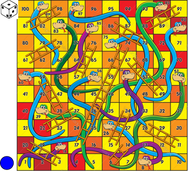
Let's play a game of Ludo to arrive at the answer.

1.1. A mathematical Ludo

A typical components of a Ludo game look like this:


A board, a die, a counter, and some rules

The Ludo we are going to play also has the same components, but is more sophisticated. The board will be the entire ${\mathbb R}^2,$ and the counter will be a single point, which is initially at $(X,Y)=(0,0).$

The die will be 4-faced, carrying the numbers 1 to 4.

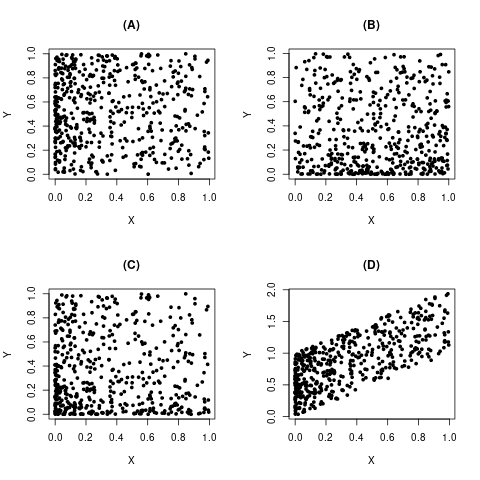
Accordingly, there are 4 rules of motion. The outcome of the die roll will determine which rule will apply at each step. The rules are:

$$\begin{eqnarray*}X_{new} & = & 0.8 X_{old}+0.1\\ Y_{new} & = & 0.8 Y_{old}+0.04\end{eqnarray*}$$
$$\begin{eqnarray*}X_{new} & = & 0.5 X_{old}+0.25\\ Y_{new} & = & 0.5 Y_{old}+0.4\end{eqnarray*}$$
$$\begin{eqnarray*}X_{new} & = & 0.355 X_{old}-0.355Y_{old}+0.266\\ Y_{new} & = & 0.355 X_{old}+0.355 Y_{old}+0.078\end{eqnarray*}$$
$$\begin{eqnarray*}X_{new} & = & 0.355 X_{old}+0.355Y_{old}+0.378\\ Y_{new} & = & -0.355 X_{old}+0.355 Y_{old}+0.434\end{eqnarray*}$$

These are all formulae to compute the new position, $(X_{new},Y_{new})$ from the old position $(X_{old},Y_{old})$ of the counter.

The game proceeds like this: The counter starts at $(X,Y)=(0,0).$ At each step the 4-faced die is rolled and the corresponding rule is applied to find the new position of the counter. The new counter position is marked with a dot after each step.

Thus, after you have played this game for, say, 10000 times, you have as many dots on the paper. What will all these dots together look like? A random jumble? A circle? A line? or what?

Make a guess and then check it by actually playing this game.

You'll be surprised by the outcome. Somehow all the randomness has vanished, and a very regular pattern has emerged!

How? Will this always happen? What if I change those formulae?

These are the questions that probability theory wants to answer.

This "regular pattern born out of randomness" phenomenon is called Statistical Regularity.

1.2. Statistical regularity

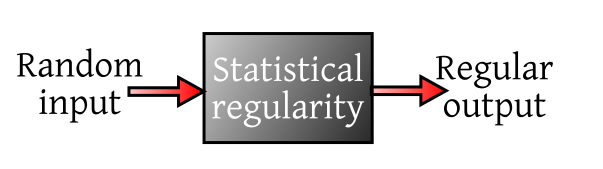
The patterns born out of statistical regularity are different from deterministic patterns in the sense that they are rarely exactly replicated. They is extremely similar, but not the same. We see this all around us. Our finger prints or the leaves on a tree furnish real life examples. Statistical regularity is like a mysterious black box which takes random unpredictable input and somehow digests the randomness to produce regular output.


Statistical regularity as a blackbox

Why do we care about statistical regularity? Firstly, because it is intriguing. Secondly, if we can master this technique, then it should help us to build robust systems that do not suffer much from randomness of inputs. The quite regular profit of a Casino or an insurance company is a familiar example.

1.3. Simplest example of statistical regularity

Statistical regularity takes many forms, some more dramatic, some less. The simplest occurrence of the phenomenon was observed long back by gamblers: If you toss a coin a large number of times, the running proportion of heads gradually stabilises. It was first proved mathematically by Jakob Bernoulli in 1713. We shall learn it in this course. He discovered the theorem and its rather short proof "after having meditated on it for twenty years"!

Try it out with a computer/phone.

2. Computer simulation (not in syllabus)

Behind every occurence of statistical regularity we have a random experiment, which we need to repeat a large number of times independently. Unfortunately, even a simple random experiment like a coin toss is difficult to be repeated many times by hand. So one prefers to use a computer to carry out a random experiment. Most computer languages and softwares have provision to program a random experiment. We shall use a software called R, which is particularly suited for this purpose. Also, it is free and easy to install. You can even run it on the cloud from your smart phone without installing anything!

To draw a Simple Random Sample Without Replacement (SRSWOR) of size 5 from the population $\{1,2,...,10\}$ you use
```
sample(10,5)
```
To draw Simple Random Sample With Replacement (SRSWR) of size $10$ from the population $\{1,2,...,6\}$ use
```
sample(6,1,replace=TRUE)
```
or, in short,
```
sample(6,1,rep=T)
```
Before you use the short form, just make sure you do not have a variable called T somewhere already. SRSWR may be used to toss coins (population of size 2) or roll dice (population of size 6). You may toss a biased coin with $P(head)=0.4$ independently 10 times by
```
sample(2,10,rep=T,prob=c(0.4,0.6))
```
Here the populaton is $\{1,2\},$ and we interpret $1$ as head. If you want make the population {head,tail}, then use
```
sample(c('Head','Tail'),10,rep=T,prob=c(0.4,0.6))
```
To generate data from some standard distribution, R provides a function starting with r followed by an abbreviated name of the distribution. For instance to generate a random sample of size 1000 from $N(0,2^2)$ distribution we use
```
rnorm(1000,mean=0,sd=2)
```
Other r-functions include rbinom, rpois, rexpo, runif rcauchy etc.

2.1. Simulating statistical regularity

Let write some R code to see statistical regularity at work. We shall simulate the coin toss example done in class: Tossing a coin a large number of times, and plotting the cumulative proportion of heads. If the first 5 outcomes are H, T, T, H, H, then the cumulative proportions are $1,\frac 12,\frac 13,\frac 24,\frac 35.$ It is always (no. of H's so far)/(no. of tosses so far). We shall plot these five proportions against (no. of tosses so far). The R command is

outcomes = sample(c('H','T'),1000,rep=T)
heads.so.far = cumsum(outcomes == 'H')
tosses.so.far = 1:1000
prop = heads.so.far/tosses.so.far
plot(prop, type='l')

Explanation of the code:

Here outcomes == "H" checks which outcomes are "H" and creates an array of 1 (yes) and 0 (no).
cumsum finds cumultative sums.
1:1000 is just the array 1,2,...,1000.
plot makes a plot. The type="l" tells it to make a line plot.

Notice how the line (which is random) jumps around a lot initially, but eventually stabilises and seems to approach a fixed value. Run the same code a number of times to see how the initial part changes drastically from run to run, but the final stable section remains unperturbed.

2.2. Problem set

The following problems will help you to enjoy the course better. However, no coding problem will be asked in the exams.

Simulate a Europian Roullette wheel. It is wheel with the numbers 0,1,...,38 written along the circumference. The wheel is spun and a ball is dropped on it. When the wheel stops spinning, the ball is at one of the numbers randomly.
Roll a fair die 5000 times. Make a line plot showing the running proportions of 6.
Suggest how you can shuffle a deck of 52 cards using R.
A slot machine consists of three reels (rings showing the numbers 0,1,...,9). When it is activated by pulling a handle the reels start turning randomly in different/same directions and stop at random positions. One digit of each reel is visible through a window. Simulate this in R.

3. Visualising density

The first topic in Probability II is transformation of multivariate densities. For this, it would help to be able to visualise both univariate and multivariate densities. This is closely relate to statistical regularity. We shall explore this visually in the 1D and 2D cases.

3.1. 1D case

A random variable is a real valued function defined on a probability space $(\Omega, \calF, P). $ You can think of the probability space as a mathematical description of a random experiment. Thus, any random variable has a random experiment behind it. Every time we carry out the random experiment, we get a random $\omega\in\Omega$ as our output, based on which compute one value $X(\omega)$ of our random variable.

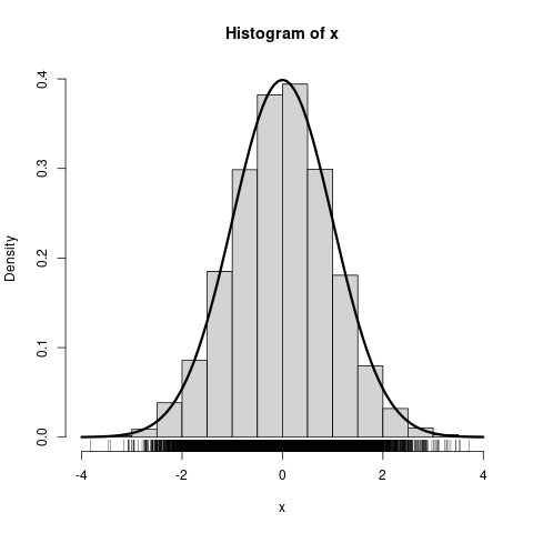
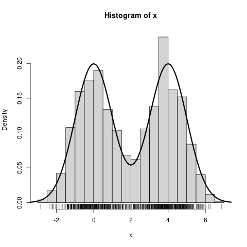
If we carry out that random experiment independently a large number of times, we shall get many values of that random variable. If we make a histogram of all those values, then the shape of that histogram approaches a particular graph. This limiting graph is called the density of the random variable. We show two examples.


An example with a single peak (unimodal)


An example with two peaks (bimodal)

The generated points themselves are shown below the histogram. Notice how they crowd together where the density peaks up. This is the reason why a density is a called "density".

3.2. 2D case

A 2D random variable (also called a 2D random vector) is just an ordered pair, $(X,Y)$, of two 1D random variables, $X$ and $Y$. The two random variables are jointly distributed, i.e., they are both defined on the same probability space, $(\Omega, \calF, P).$ Recall that the probability space is just a random experiment. When we run that experiment, we get some outcome $\omega\in \Omega.$ Based on that same $\omega$ we compute $X(\omega)$ and $Y(\omega).$ So each time you run the experiment, you get a point, $(X(\omega),Y(\omega))$, that you can plot on a graph paper. When we run the experiment a large number of times independently, you get a spray of points. As before, the density of the spray may be different at different parts of the $xy$-plane. This varying level of concentration is captured by the (joint) density of $(X,Y).$

EXAMPLE 1:

A bivariate density

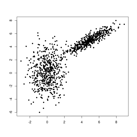
Scatterplot from it

Observe how the random points crowd more densely near the peaks. ■

A special case that will occur frequntly in our discussions is $Unif(S)$ for a bounded subset $S\subseteq{\mathbb R}^2.$ Here the density is a $\frac{1}{area(S)}$ over $S$ (and 0 outside). If we draw a random point from this density, the point must lie inside $S$ and is equally likely to land anywhere in $S.$

3.3. Problem set

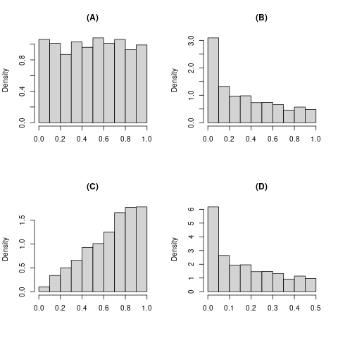
EXERCISE 1: I have a random sample of size 1000 from the $Unif(0,1)$ distribution. If I square all the numbers in my sample then which of the following is most likely to be shape of the resulting histogram?

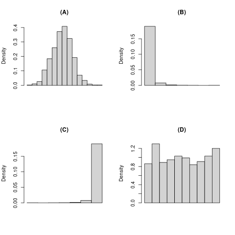
EXERCISE 2: Sppose that we collect data on the monthly income of all Indians, and make a histogram of the resulting data. Which of the following shapes would you expect?

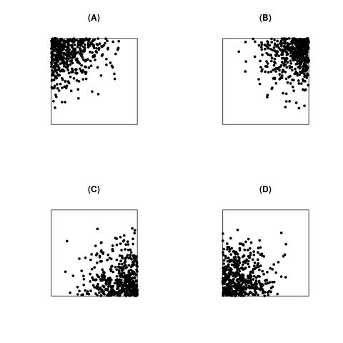
EXERCISE 3: Consider the joint density $$f(x,y) = \left\{\begin{array}{ll}9x^2y^2&\text{if }0\leq x,y\leq 1\\ 0&\text{otherwise.}\end{array}\right..$$ If we generate data from it, which of the following scatterplots would the data most likely correspond to?


In each case, the box is the unit square.

[Hint]

The density looks like this:

EXERCISE 4: A bivariate density $f(x,y)$ is actually free of $y.$ Then which of the following scatterplots is most likely to be generated by it?