 |
|---|
| Some $\k k$ densities |
| Last updated on: Mon Sep 28 18:25:54 IST 2026 |
Proof:Only if part: Take $A = I_d$ and $\v \mu = \v 0_{d\times 1}.$ Then by the above definition $$A\v X + \v \mu = \v X\sim N_d(\v 0, I),$$ because $AA' = I.$
If part: Shall do later in the final section of this page. [QED]Proof: Let us take some matrix $A$ for which $\Sigma = AA'.$ Also we take a random vector $\v Z$ whose components are iid $N(0,1).$
Let $\v Y = \v \mu + A\v Z.$ Then $\v Y$ and $\v X$ has the same distribution. So enough to show $E(\v Y)=\v \mu$ and $V(\v Y) = \Sigma.$ We have $E(\v Z) = \v 0$ and $V(\v Z) = I.$ So $E(\v Y) = \v \mu + A E(\v Z) = \v \mu$ and $V(\v Y) = A V(\v Z)A' = AA' = \Sigma.$ [QED]Proof: Let us take some matrix $A$ for which $\Sigma = AA'.$ Also we take a random vector $\v Z$ whose components are iid $N(0,1).$
Let $\v Y = \v \mu + A\v Z.$ Then $\v Y$ and $\v X$ has the same distribution. So enough to show $B\v Y+\v c\sim N_r(B\v\mu+\v c, B \Sigma B').)$ Now $B\v Y + \v c = B(\v \mu + A\v Z) +\v c= B\v \mu+\v c + BA\v Z\sim N_r(B\v \mu+\v c,BAA'B')\equiv N_r(B\v \mu+\v c,B \Sigma B'),$ as required. [QED] We can easily compute the marginals of a multivariate normal distribution using this theorem.EXAMPLE 1: Let $\v X = \left[\begin{array}{ccccccccccc}X\\Y\\Z \end{array}\right]\sim N_3\left(\left[\begin{array}{ccccccccccc}1\\2\\3 \end{array}\right],\left[\begin{array}{ccccccccccc}2 & 0 & 1\\0 & 20 & 2\\1 & 2 & 100 \end{array}\right]\right).$ Find the distributions of $Y$ and $(X,Z).$
SOLUTION: Take $B = \left[\begin{array}{ccccccccccc}0 & 1 & 0 \end{array}\right].$ Then $B\v X = Y\sim N(2,20).$ Again, taking $B = \left[\begin{array}{ccccccccccc}1 & 0 & 0\\0 & 0 & 1 \end{array}\right]$, we have $B\v X = \left[\begin{array}{ccccccccccc}X\\Z \end{array}\right]\sim N_2\left(\left[\begin{array}{ccccccccccc}1\\3 \end{array}\right],\left[\begin{array}{ccccccccccc}2 & 1\\1 & 100 \end{array}\right]\right)$. ■ Thus, we see that the various marginals are also normal with the "corresponding" parts of the original mean vector and covariance matrix.Proof:Will be done in the final section of this page.[QED]
EXERCISE 1: Find the distribution of $Y.$
EXERCISE 2: Find the distribution of $(X,Z).$
EXERCISE 3: Find the distribution of $(X+Y,X+W).$
EXERCISE 4: If $X_1,X_2,X_3$ are iid $N(0,1),$ then show that $X_1+X_2+X_3$ and $X_1-2X_2+X_3$ are independent.
EXERCISE 5: If $\v X\sim N_d(\v \mu, I)$ and $\v a, \v b\in{\mathbb R}^d$ are two fixed vectors with $\v a'\v b = 0$ (i.e., they are orthogonal to each other), then show that $\v a'\v X$ and $\v b'\v X$ are independent.
EXERCISE 6: Show that $N_d(\v 0, I)$ has joint density $f(\v x) = (2\pi)^{-\frac d2} e^{-\frac 12\v x'\v x} $ for $\v x\in{\mathbb R}^d.$
Hint:
The components are iid $N(0,1)$. Multiply their densities.
EXERCISE 7: Show that if $\Sigma$ is pd, then $N_d(\v \mu, \Sigma)$ has density $$f(\v x) = (2\pi det(\Sigma))^{-\frac 12} e^{-\frac 12(\v x-\v \mu)' \Sigma ^{-1}(\v x-\v \mu) } \mbox{ for }\v x\in{\mathbb R}^d.$$
Proof: Note that $\bar X$ is a linear combination of $X_1,...,X_n.$ So $\bar X$ must be a normal random variable. Its parameters will be $$E(\bar X) = E\left(\frac 1n\sum_1^n X_i\right) = \frac 1n(\underbrace{\mu+\cdots+\mu}_{n\mbox{ times}}) = \mu,$$ and $$V(\bar X) = V\left(\frac 1n\sum_1^n X_i\right) = \frac{1}{n^2}(\underbrace{\sigma^2+\cdots+\sigma^2}_{n\mbox{ times}}) = \frac{\sigma^2}{n},$$ since the $X_i$'s are independent (making the covariance terms zero).
This completes the proof. [QED] |
|---|
| Some $\k k$ densities |
Proof:(Induction on $k$):
Basis: For $k=1$, we have $S_1^2 = \sum_{i=1}^1 (x_1-\bar x_1)^2 = 0,$ since $\bar x_1 = x_1.$ Also the rhs is a sum from $i=1$ to $0 (< 1),$ and hence is 0. Hypothesis: We assume the result for $k=1,2,...,n$ for some $n\geq 1.$ Step: Shall show the result for $k=n+1.$ Now $$\begin{eqnarray*} S_{n+1}^2 & = & \sum_{i=1}^{n+1} (X_i-\bar X_{n+1})^2\\ & = & \sum_{i=1}^{n+1} \left(X_i-\frac{n\bar X_n+X_{n+1}}{n+1}\right)^2\\ & = & \sum_{i=1}^{n+1} \left(\underbrace{X_i-\bar X_n}_a - \underbrace{\frac{X_{n+1}-\bar X_n}{n+1}}_b\right)^2\mbox{(Be careful!)}\\ & & \mbox{Applying $(a-b)^2$ formula,}\\ & = & \sum_{i=1}^{n+1} \left[ (X_i-\bar X_n)^2 + \frac{(X_{n+1}-\bar X_n)^2}{(n+1)^2} -2 \frac{(X_i-\bar X_n)(X_{n+1}-\bar X_n)}{n+1} \right]\\ & = & \sum_{i=1}^{n+1} (X_i-\bar X_n)^2 + \frac{(X_{n+1}-\bar X_n)^2}{n+1} -\frac{2(X_{n+1}-\bar X_n)}{n+1} \sum_{i=1}^{n+1}(X_i-\bar X_n) \\ & = & \big[S_n^2+ (X_{n+1}-\bar X_n)^2\big] + \frac{(X_{n+1}-\bar X_n)^2}{n+1} -\frac{2(X_{n+1}-\bar X_n)}{n+1} (X_{n+1}-\bar X_n)~~\left[\mbox{$\because\sum_1^n (X_i-\bar X_n)=0.$}\right] \\ & = & S_n^2+ (X_{n+1}-\bar X_n)^2 - \frac{(X_{n+1}-\bar X_n)^2}{n+1} \\ & = & S_n^2+ \frac{n}{n+1}(X_{n+1}-\bar X_n)^2. \end{eqnarray*}$$ Now, by the induction hypothesis, we have $$S_n^2 =\sum_{i=1}^{n-1} \frac{i}{i+1}(x_i-\bar x_n)^2.$$ So we have $$S_{n+1}^2 =\sum_{i=1}^{n-1} \frac{i}{i+1}(x_i-\bar x_n)^2+\frac{n}{n+1}(X_{n+1}-\bar X_n)^2 = \sum_{i=1}^n \frac{i}{i+1}(x_i-\bar x_n)^2,$$ as required. So the result is proved by the principle of mathematical induction. [QED] Now we are in a position to prove Theorem 2. Proof of Theorem 2: The theorem expresses $S_n^2$ as $\sum_{i=1}^{n-1} U_i^2,$ where $U_i = \sqrt{\frac{i}{i+1}} (X_{i+1}-\bar X_i).$ Hence the required $\k{n-1}$ distribution will be proved once we show that $U_1,...,U_{n-1}$ are iid $N(0,1).$ Notice that the $U_i$'s are all linear combinations of $X_1,...,X_n.$ So $(U_1,...,U_{n-1})'$ has a multivariate normal distribution. So enough to show that $E(U_i) = 0$, $V(U_i) = 1$ and for $i\neq j$ $\cov(U_i,U_j) = 0.$Proof: In the last proof we showed that $S^2$ is a function of $U_1^2,...,U_{n-1}^2.$
So it is enough to show that $\bar X$ is independent of $(U_1,...,U_{n-1}).$ Since $\bar X$ as well as the $U_i$'s are linear combinations of $X_1,...,X_n,$ hence $(\bar X,U_1,...,U_{n-1})$ has multivariate normal distribution. So to prove independence, it is enough to show that $\cov(\bar X, U_i) = 0$ for $i=1,...,n-1.$ Now $$\begin{eqnarray*} \cov(\bar X, U_i) & = & \sqrt{\frac{i}{i+1}}\cov(\bar X, X_{i+1}-\bar X_i)\\ & = & \sqrt{\frac{i}{i+1}}\big[\cov(\bar X, X_{i+1})-\cov(\bar X,\bar X_i) \big]\\ & = & \sqrt{\frac{i}{i+1}}\left[ \frac 1n\cov(X_1+\cdots X_n, X_{i+1})-\frac{1}{ni}\cov(X_1+\cdots+X_n,X_1+\cdots+\cdots X_i) \right]\\ & = & \sqrt{\frac{i}{i+1}}\left[ \frac{\sigma^2}{n}-\frac{\sigma^2}{n} \right] = 0, \end{eqnarray*}$$ as required. [QED]EXERCISE 8: If $X_1,...,X_{100}$ are iid $N(3,4^2),$ then what is the sampling distribution of sample mean?
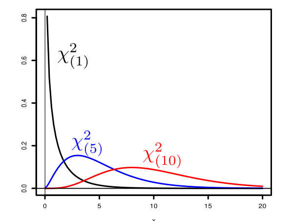
EXERCISE 9: If $(X_1,...,X_{100})$ is a random sample from $N(3,2^2),$ then what is the probability that the sample variance exceeds 5? Express your answer in terms of $F_k(x)$, the distribution function of $\k k$ distribution. Assume that the sample variance is computed with $n-1$ in the denominator.
EXERCISE 10: If $X_1,...,X_n$ are iid $N(2,3^2).$ Find $P(\bar X \in (1,3))$ in terms of the standard normal distribution function $\Phi(\cdot).$
EXERCISE 11: If $X_1,X_2,...$ are iid $N(0,1)$ and $\bar X_n = \frac 1n\sum_1^n X_i$ and $S_n^2 = \sum_1^n (X_i-\bar X_n)^2,$ then which of the following statements is/are true?
EXERCISE 12: $X_i$ s iid $N(0,1).$ What will the distribution of $\sum_1^n (X_i-a)^2$ be, where $a\in{\mathbb R}$ is a fixed number?
 |
|---|
| Some $t$-densities |
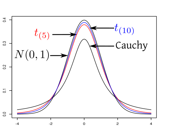
EXERCISE 13: Consider the density of $t_{(k)}$-distribution. Do you recognise the $t_{(1)}$-distribution as something already familiar?
EXERCISE 14: Let $X_1,...,X_n$ be a random sample from $N(\mu,\sigma^2).$ Then what is the distribution of $$\frac{\sqrt n(\bar X-\mu)}{\sqrt{\sum(X_i-\bar X)^2/(n-1)}}?$$
EXERCISE 15: Let $X_1,...,X_{100}$ be a random sample from $N(\mu,\sigma^2).$ Find $a>0$ such that $P(\mu\in (\hat \mu-a \hat \sigma^2,\hat \mu+a \hat \sigma^2)) = 0.95,$ where $\hat \mu$ is the sample mean and $\hat \sigma^2$ is the sample variance (with $n-1$ in the denominator). Express your answer in terms of the distribution function, $F_k(\cdot)$ of the $t_{(k)}$-distribution.
 |
|---|
| Some $F$-densities |
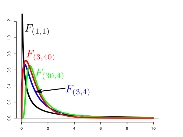
EXERCISE 16: Let $X_1,...,X_m$ and $Y_1,...,Y_n$ be random samples from $N(\mu_1,\sigma^2)$ and $N(\mu_2,\sigma^2)$, respectively (same $\sigma^2$). Then what is the distribution of $$\frac{\sum(X_i-\bar X)^2/(m-1)}{\sum(Y_i-\bar Y)^2/(n-1)}?$$
EXERCISE 17: If $X\sim t_{(1)},$ then what is the distribution of $X^2?$
EXERCISE 18: If $X\sim F_{(2,3)},$ then what is the distribution of $\frac 1X?$
Proof:Not to be done in this course.[QED]
Proof: $$\begin{eqnarray*} M_{\v X+\v Y}(\v t) & = & E(e^{\v t'(\v X + \v Y)})\\ & = & E(e^{\v t'\v X}e^{\v t'\v Y)})\\ & = & E(e^{\v t'\v X})E(e^{\v t'\v Y})~~\left[\mbox{$\v X, \v Y$ independent}\right]\\ & = & M_X(\v t)M_Y(\v t). \end{eqnarray*}$$ [QED]
Proof: $$\begin{eqnarray*} M_{\v Z} (\v s, \v t) & = & E\left[\exp\left(\left[\begin{array}{ccccccccccc}\v s' & \v t' \end{array}\right]\left[\begin{array}{ccccccccccc}\v X\\\v Y \end{array}\right] \right) \right]\\ & = & E(e^{\v s'\v X}e^{\v t'\v Y)})\\ & = & E(e^{\v s'\v X})E(e^{\v t'\v Y})~~\left[\mbox{$\v X, \v Y$ independent}\right]\\ & = & M_X(\v s)M_Y(\v t). \end{eqnarray*}$$ [QED]
EXERCISE 19: If $X_1,X_2,X_3$ are iid $N(0,1),$ then find the mgf $M(\v t)$ of $\v X = \left[\begin{array}{ccccccccccc}X_1\\X_2\\X_3 \end{array}\right].$
Hint:
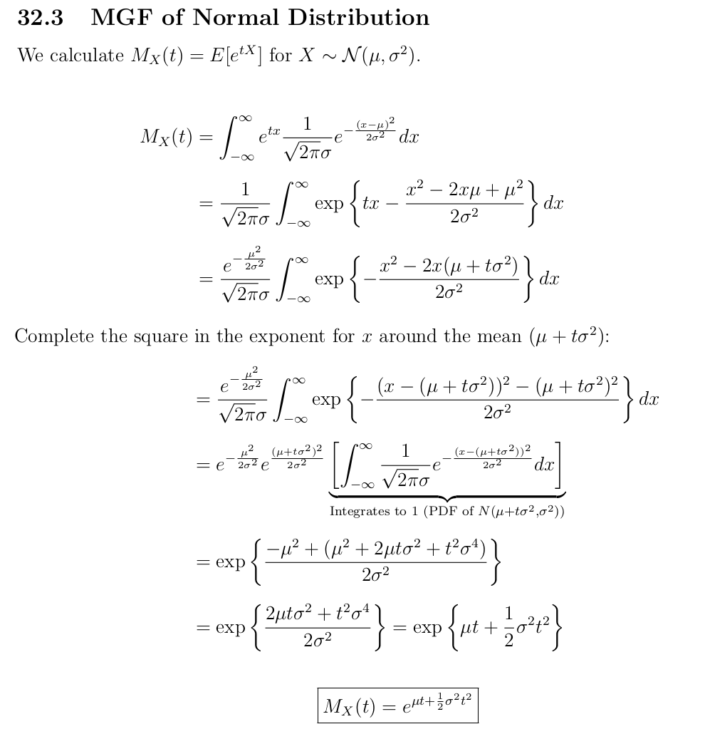
$N(0,1)$ has mgf $e^{t^2/2}$ for $t\in{\mathbb R}.$
EXERCISE 20: Find the mgf of $N_d(\v 0, I)$ distribution.
EXERCISE 21: If $\v X_{d\times 1}$ has mgf $M(\v t)$, then find the mgf of $A\v X+\v b$ where $A_{n\times d}$ and $\v b_{n\times 1}$ are fixed.
Proof: Recall from Probability I that mgf of each $X_i$ is $E(e^{sX_1})=e^{s^2/2}$ for $s\in{\mathbb R}.$
So the mgf of $\v X = (X_1,...,X_n)'$ is $$\begin{eqnarray*} M_{\v X}(\underbrace{s_1,...,s_n}_{\v s})=E(e^{s_1X_1+\cdots+s_nX_n}) & = & E(e^{s_1X_1})\cdots E(e^{s_nX_n}) ~~\left[\mbox{$\because$independent}\right] \\ & = & e^{\frac 12(s_1^2+\cdots+s_n^2)} = e^{\v s'\v s/2} \end{eqnarray*}$$ for all $\v s=(s_1,...,s_n)'\in{\mathbb R}^n.$ So mgf of $\v Y = A\v X + \v b$ is $$\begin{eqnarray*} M_{\v Y}(\v t) & = & E(e^{\v t'(A\v X+\v b)})\\ & = & E(e^{\v t'A\v X+\v t'\v b})\\ & = & e^{\v t'\v b}E(e^{\v t'A\v X})\\ & = & e^{\v t'\v b}E(e^{(A'\v t)'\v X})\\ & = & e^{\v t'\v b}e^{(A'\v t)'(A'\v t)/2}\\ & = & e^{\v t'\v b+\v t' AA'\v t/2}, \end{eqnarray*}$$ as required. [QED] Since the MGF is defined over a neighbourhood of the origin (in fact everywhere), the MGF characterises the distribution. Thus, the distribution is characterised by $\v b$ and $AA'.$ Thus, we have also proved:Proof:Let $\{\v e_1,...,\v e_n\}$ be the canonical basis. Then for $i\in\{1,...,n\}$ we have $\v e_i'A\v e_i = \v e_i'B\v e_i$, or $a_{ii} = b_{ii}.$
Similarly, $\forall i,j\in\{1,...,n\}$ if we take $\v x = \v e_i+\v e_j,$ then $\v x'A\v x = \v x' B\v x$, or $$a_{ii}+a_{ij}+a_{ji}+a_{jj}=b_{ii}+b_{ij}+b_{ji}+b_{jj}.$$ Since the diagonal entries match, have $a_{ij}+a_{ji}=b_{ij}+b_{ji}.$ Since $A,B$ are symmetric, hence this forces $a_{ij} = b_{ij}.$ [QED]Proof:We already know that $X_i\sim N(\mu_i, \sigma_{ii}),$ where $\mu_i$ is the $i$-th entry of $\v \mu,$ and $\sigma_{ii}$ is the $i$-th diagonal entry of $\Sigma.$
So mgf of $X_i$ is $M(t) = e^{t \mu_i + \sigma_{ii} t^2/2}$ for $t\in{\mathbb R}.$ If the $X_i$ s were independent, then the mgf of $\v X$ would have been $M(t_1)\cdots M(t_d) = e^{\v t' \v\mu +\frac 12\v t' diag(\Sigma)\v t}$ for $\v t\in{\mathbb R}^d,$ where $diag(\Sigma)$ is the diagonal part of $\Sigma.$ Also mgf of $\v X$ is $e^{\v t'\v \mu + \frac 12\v t'\Sigma\v t}$ for $\v t\in{\mathbb R}^d.$ Thus, $X_i$ s are independent iff $$e^{\v t'\v \mu + \frac 12\v t'\Sigma\v t} = e^{\v t' \v\mu +\frac 12\v t' diag(\Sigma)\v t},$$ and this must hold for all $\v t\in{\mathbb R}^d.$ So we must have $\v t'\Sigma\v t=\v t'diag(\Sigma)\v t.$ Since $\Sigma$ is symmetric, hence the fact from linear algebra forces $\Sigma=diag(\Sigma),$ i.e., $\Sigma$ must be a diagonal matrix, as required. [QED]Proof: It should be clear that DEFN1 implies DEFN2.
To see the converse, suppose that $\v X$ has a multivariate normal distribution according to DEFN2. Then taking $\v \ell = \v e_1,...,\v e_d,$ we see that the components $X_1,...,X_d$ are all univariate normal, and so have finite second moments. Hence we can take $\v \mu = E(\v X)$ and $\Sigma = V(\v X).$ Step 1: Shall show that $\v X$ has characteristic function $\xi(\v t) = e^{i\v t'\v \mu-\frac 12\v t' \Sigma \v t}.$ From the given condition, the characteristic function of $\v \ell'\v X$ is $E(e^{i t \v \ell'\v X}) = \xi(t\v \ell),$ which must be of the form $e^{it \mu(\ell)- \frac{t^2 \sigma^2(\ell)}{2}}$ for some function $\mu(\cdot)$ and $\sigma^2(\cdot) \geq0.$ So we have $$\xi(t\v \ell) = e^{it \mu(\ell)- \frac{t^2 \sigma^2(\ell)}{2}}.$$ Since this must be the characteristic function of $N(\v \ell' \mu, \v \ell' \Sigma \v \ell),$ hence $\mu(\v \ell) = \v \ell' \v \mu$ and $\sigma^2(\v \ell) = \v \ell' \Sigma \v \ell,$ completing Step 1. Step 2: Shall show that $X-\v \mu\in\col(\Sigma)$ with probability 1. We have $\forall \v\ell\in{\mathbb R}^d~~\v \ell'\v X\sim N(\v \ell'\v \mu,\v\ell'\Sigma \v\ell).$ Now consider a basis $\{\v\ell_1,...,\v\ell_k\}$ of the orthogonal complement of $\col(\Sigma).$ Then $V(\v\ell_j'(\v X-\v \mu)) = 0$ for each $j=1,...,k.$ So $\exists \Omega_j\subseteq \Omega~~P(\Omega_j)=1~~\forall \omega\in \Omega_j~~\v\ell'(\v X(\omega)-\v \mu)=0.$ Let $\Omega_* = \Omega_1\cap\cdots\cap \Omega_k.$ Then $P(\Omega_*)=1$ and $\forall \omega\in \Omega_*~~\v X(\omega)-\v \mu\in\col(\Sigma).$ This completes Step 2. Step 3: Shall manufacture $\v Z$ to be used in DEFN1. Let $A$ be any full column rank matrix such that $\Sigma = AA'.$[Always exists. Why?...]Then $\col(A) = \col(\Sigma).$Consider spectral decomposition of $\Sigma$ with nonzero eigenvalues listed first. Make $A$ with the corresponding eigenvectors as columns.
[Because...]So, $\forall \omega\in \Omega_*$ we have $$\begin{eqnarray*} & & \v X(\omega)-\v \mu\in \col(A)\\ &\mbox{or} & \exists Z(\omega)~~\v X(\omega) -\v \mu= A \v Z(\omega)\\ &\mbox{or} & \v Z(\omega) = A^{-l}(\v X(\omega)-\v \mu). \end{eqnarray*}$$ Define $\v Z(\omega) = \v0$ for $\omega\not\in \Omega_*.$ Using the characteristic function derived in Step 1, we have $\v Z\sim N_r(\v0, I_r),$ completing the proof. [QED] Just note that what I have shown is this: If $\v X$ has multivariate normal distribution according to DEFN2, then there is a $\v Z$ with iid $N(0,1)$ components such that $\v X = \v \mu + A\v Z$ with probability 1. Indeed, there is no way I can guarantee this for all $\omega\in \Omega.$$\col(\Sigma)$ is a subspace of $\col(A)$ and $r(\Sigma)=r(A).$
EXERCISE 22: $(X,Y)$ has mgf $$M(s,t) = \exp(s-t+20s^2+42t^2-12st)\mbox{ for }(s,t)\in{\mathbb R}^2.$$ Find the distribution of $(X,Y).$
EXERCISE 23: Write the density of $X$ if it has mgf $M(t) = \exp(2t+3t^2)$ for $t\in{\mathbb R}.$