 |
|---|
| Last updated on: Wed Aug 19 12:37:28 IST 2026 |
| Last updated on: Wed Aug 19 12:37:29 IST 2026 |
Proof: Case 1: $V(X)=0$: Then $X$ is a constant (say $c$) with probability 1. So $E(X)=c.$
In this case, $$\cov(X,Y) = E\big( (X-E(X))(Y-E(Y)) \big) = E\big( (c-c) (Y-E(Y)) \big) = 0,$$ and so the inequality holds trivially (both sides being 0). Case 2: $V(Y)=0$: Similar to Case 1. Case 3: $V(X), V(Y)>0$: Define $Z_1 = \frac{X-E(X)}{\sqrt{V(X)}}$ and $Z_2 = \frac{Y-E(Y)}{\sqrt{V(Y)}}.$ Notice that $E(Z_1^2) = E(Z_2^2) = 1$ and $E(Z_1Z_2) = \frac{\cov(X,Y)}{\sqrt{V(X)V(Y)}}.$ Now $$\begin{eqnarray*} & & E(Z_1\pm Z_2)^2 \geq 0\\ &\mbox{or } & E(Z_1^2) + E(Z_2^2) \pm 2E(Z_1Z_2) \geq 0\\ &\mbox{or } & 1 + 1 \pm \frac{2\cov(X,Y)}{\sqrt{V(X)V(Y)}}\geq 0\\ &\mbox{or } & 1 \pm \frac{\cov(X,Y)}{\sqrt{V(X)V(Y)}}\geq 0\\ &\mbox{or } & \pm \frac{\cov(X,Y)}{\sqrt{V(X)V(Y)}}\leq 1\\ &\mbox{or } & \left(\frac{\cov(X,Y)}{\sqrt{V(X)V(Y)}}\right)^2\leq 1\\ &\mbox{or } & \cov(X,Y)^2\leq V(X)V(Y), \end{eqnarray*}$$ as required. Also equality holds iff $V(Z_1+Z_2)=0$ or $V(Z_1-Z_2)=0$, i.e., if $Z_1+Z_2$ or $Z_1-Z_2$ is a constant with probability 1. So we have either $P(Z_1+Z_2=k)=1$ or $P(Z_1-Z_2=k)=1$ for some $k\in{\mathbb R}.$ In both cases we have $P(aX+bY=c)=1$ for some constants, $a,b,c,$ as required. [QED] It is instructive to think about the Cauchy-Schwarz inequality from a geometric perspective. If we take two vectors , $\v u$ and $\v v$ in 2D or 3D, we have the identity $$\v u\bullet\v v = \| \v u\| \cdot \|\v v\|\cos \theta,$$ where $\theta$ is the angle between the two vectors. |
|---|
EXERCISE 1: Let $V(X) = 2$, $V(Y) = 4.5$ and $\cov(X,Y) = -3.$ If $E(X) = 1$, $E(Y) = 2,$ then find $a,b,c\in{\mathbb R}$ such that $P(aX+bY=c)=1.$
Hint:
Here equality holds in Cauchy-Schwarz inequality. Define $Z_1,Z_2$ as in the proof of Cauchy-Schwarz inequality. Either $V(Z_1+Z_2)=0$ or $V(Z_1-Z_2)=0.$ Which one?
EXERCISE 2: Here is another variant of the Cauchy-Schwarz inequality:
If $X,Y$ are jointly distributed random variables with $E(X^2),E(Y^2) < \infty,$ then $E^2(XY)\leq E(X^2)E(Y^2).$Prove this.
Hint:
Just mimick the proof above. Cases 1 and 2 for $E(X^2)=0$ and $E(Y^2)=0.$ In case 3 take $Z_1=\frac{X}{\sqrt{E(X^2)}}$ and $Z_2=\frac{Y}{\sqrt{E(Y^2)}}.$
EXERCISE 3: $X$ is a nonnegative random variable with finite second moment. Show that $P(X>0)\geq \frac{E^2(X)}{E(X^2)}.$
Hint:
Take $Y = \left\{\begin{array}{ll}1&\text{if }X>0\\ 0&\text{otherwise.}\end{array}\right..$ Apply the form of Cauchy-Schwarz inequality in the last exercise.
EXERCISE 4: Let $X_1,...,X_n$ be random variables with finite second moments. Show that $$V\left(\sum X_i\right) \leq \left(\sum\sqrt{V(X_i)}\right)^2.$$
EXERCISE 5: Show that $E|X-E(X)|\leq \sqrt{V(X)}$ for any random variable $X$ with finite second moment.
EXERCISE 6: If $E(X^2)=E(Y^2) = E(XY),$ then show that $P(X=Y)=1.$
EXAMPLE 1: 10 nonnegative numbers have a total of 100. Three of the numbers are $\geq 35$. Can this statement be true?
SOLUTION: No, because just these three numbers already have a total exceeding 100. Since the other numbers are nonnegative, they cannot bring the total down! You can think of it as trying to satisfy the given conditions using the smallest possible numbers: |
|---|
EXAMPLE 2: Average salary in a company is Rs 50,000. It is claimed that 30% of the employees are getting salaries $\geq$Rs 2,50,000. Can this claim be true?
SOLUTION: Again consider the smallest possible numbers subject to the given conditions: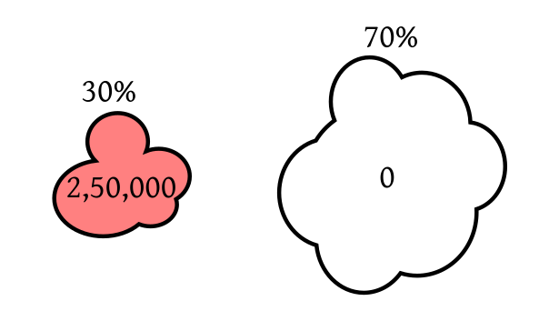 |
|---|
Proof: As in the examples above, we consider the "minimum possible version of $X$": $$Y = \left\{\begin{array}{ll} \epsilon&\text{if }X\geq \epsilon\\ 0&\text{otherwise.}\end{array}\right..$$ We must have $Y\leq X.$ Hence $E(Y)\leq E(X).$ But $E(Y) = P(X\geq \epsilon) \epsilon.$ Hence the result. [QED]
A point about the inequalities in the above theorem. There are two inequalities, one inside the probability, and one outside: $$P(X \geq \epsilon) \leq \frac{E(X)}{\epsilon}.$$ Both are mixed inequalities. Obviously, you may make the first inequality strict (thereby weakening the result). However, you may not replace the other inequality with a strict one, because otherwise you will get $1 < 0$ for the degenerate random variable $X\equiv0$. The following variant of the Markov inequality is due to Chebyshev.| Chebyshev is also credited with designing a quadruped robot-like linkage. |
Proof: Note that $P(|X-E(X)| \geq \epsilon) = P((X-E(X))^2 \geq \epsilon^2).$ Now apply Markov inequality to the random variable $(X-E(X))^2.$ [QED]
EXERCISE 7: Give a counterexample to show that the nonnegativity assumption in the inequality may not be dropped.
EXERCISE 8: Let $X$ be any random variable (not necessarily nonnegative). Show that $$\forall \epsilon>0~~P(X\geq \epsilon) \leq \frac{E(X^2)}{\epsilon^2}.$$
EXERCISE 9: If you have solved the above exercise, you can also show that for any nonnegative random variable $X$ and any $\epsilon>0$ we have for each $k\in{\mathbb N},$ $$\forall \epsilon>0~~P(X\geq \epsilon) \leq \frac{E(X^k)}{\epsilon^k}.$$ Will higher values of $k$ necessarily give you better bounds?
EXERCISE 10: Prove that $\forall \epsilon>0~~\frac{1}{\sqrt{2\pi}}\int_{-\epsilon}^ \epsilon e^{-x^2/2}\, dx \geq \frac{\epsilon^2-1}{\epsilon^2}.$
Here we sort an array of numbers by picking a random element from the array, and dividing the rest into two groups, depending on whether a number is $\leq$ or $>$ than the picked element. Then we do the same thing recursively to both the groups separately, and stop when the entire array is sorted.Let $X$ denote the number steps in a Las Vegas algorithm. We often know $E(X)$ as a function of the input size. For instance, in the randomised quicksort algorithm $E(X) = n\log n,$ where $n$ is the length of the array (proof not part of this course). Then Markov inequality helps us to get an upper bound on the probability that the algorithm will take too long. This allows engineers to guarantee system stability without knowing the exact distribution of $X.$
EXERCISE 11: Let $X$ be the number of steps needed in a randomised quick sort algorithm. It is known that $E(X)=n\log n$ if the $n$ is the length of the array to be sorted. Find an upper bound for $P(X>10^6)$ if the input array has length $10^4.$
EXERCISE 12: (Router overload) A router receives a random number ($X$) of packets every millisecond. We know from the past that $E(X)=50.$ We do not know the distribution of $X.$ The router's buffer can hold 250 packets before overflowing. Help the network engineer to provide an uppr bound to the failure rate, $P(X\geq 250).$
EXERCISE 13: (Liquidity crisis) A bank has a large portfolio of small business loans. $X=$ number of defaulters in a single month. Past experience shows $E(X)=2M.$ Liquidity crisis will arise if $X\geq 20M.$ Bound the probability of that.
EXERCISE 14: (System downtime) A financial system tracks $X$ the downtime of the system per year. Past data shows $E(X)=15$ minutes. Crash would result if $X\geq 2$ hours. Bound its probability.
EXERCISE 15: (Volatile market) When the market is highly volatile market, an investment fund's historical data becomes useless. The only certain information is the current daily expected loss $E(X)=100,000.$ Upper bound $P(X\geq 1,000,000).$
EXERCISE 16: (Primality testing) A randomised primality testing algorithm called the Miller Rabin test applies a random experiment on an input integer $n.$ The (random) output is either "Composite" or "Prime". There is theoretical guarantee that if it says "Composite", then the input is indeed composite. But if it says "Prime" then the input is composite with 0.25 probability.
Mathematically, let $$X = \left\{\begin{array}{ll}1&\text{if }\mbox{error}\\ 0&\text{otherwise.}\end{array}\right..$$ Then we have $E(X) = \frac 14.$ We run this experiment $k$ times independently (on the same input), and we output "Composite" if at least one run says so. Otherwise, we say "Prime". Give an upper bound on the probability that this battery of $k$ tests makes an error. [This problem can also be solved without explicit use of Markov inequality.]