$\newcommand{\v}[1]{\boldsymbol{#1}}$
$\newcommand{\io}{~~\mathrm{i.o.}}$
$\newcommand{\calF}{\mathcal{F}}$
$\newcommand{\rightarrowL}[1]{\stackrel{L_{#1}}{\longrightarrow}}$
$\newcommand{\rightarrowP}{\stackrel{P}{\longrightarrow}}$
$\newcommand{\rightarrowD}{\stackrel{d}{\longrightarrow}}$
$\newcommand{\rightarrowA}{\stackrel{a.s.}{\longrightarrow}}$
Convergence of random variables
The main theme of probability theory is exploring statistical regularity. This phenomenon is all about
the limiting behaviour
of a sequence of random variables. So it is only natural that convergence of random variables
occupies a central position in probability theory. What is surprising, however, is that a sequence random variables may
converge in many different ways. So there is no single definition of a "limit of a sequence of
random variables". In this page we shall define 4 different notions of convergence of a sequence of random variables:
Almost sure convergence
convergence in probability
convergence in distribution
$L_p$ convergence
Each captures one aspect of our intuitive idea about convergence of random variables.
Since random variables are just functions (from a probability space $(\Omega,\calF,P)$ to
${\mathbb R}$), the very first definition of convergence
that comes to our mind is pointwise convergence, i.e., we want
However, we also know that random variables are used only in probability computation, and so if we take some $A\subseteq \Omega$
such that $P(A)=0,$ then the behaviour of a random variable over $A$ "does not really matter".
Hence instead of wanting to have $X_n(\omega)\rightarrow X(\omega)$ everywhere (i.e., $\forall \omega\in
\Omega$) it is enough to have it almost everywhere (i.e., $\forall \omega\in$ a set of probability 1).
EXAMPLE 1: Let our probability space be $Unif[0,1]$ with $\Omega = {\mathbb R}.$ Let $X_n(\omega)
=\omega^n$, and let $X(\omega)\equiv 0.$
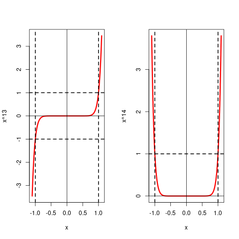
Then the event $\{X_n\rightarrow X\}$ is the set of all $\omega$ such that $X_n(\omega)\rightarrow X(w)$, which is $(-1,1).$
Let's understand this with some examples. We shall consider different values of $\omega\in{\mathbb R}$ and see when $X_n(\omega) \rightarrow X(\omega)$
holds, i.e., when $\omega^n\rightarrow 0$ holds.
If $\omega=\frac 12,$ then $\omega^n = \left(\frac 12\right)^n\rightarrow 0.$ More generally, for
all $\omega\in[0,1)$ we have $\omega^n \rightarrow 0.$
If $\omega = -\frac 12,$ then also $\omega^n = \left(-\frac 12\right)^n\rightarrow 0,$ and in
general, for all $\omega\in(-1,0)$ we have $\omega^n \rightarrow 0.$
If $\omega = 1,$ then $\omega^n=1^n = 1 \rightarrow 1,$ and hence $\omega^n \not\rightarrow 0.$
If $\omega=2,$ then $\omega^n = 2^n\rightarrow \infty,$ and hence again $\omega^n
\not\rightarrow 0.$ More generally, for all $\omega > 1,$ we have $\omega^n \not\rightarrow 0.$
If $\omega = -2,$ then $\omega^n$ keeps on oscillating, and does not converge. So
here also $\omega^n \not\rightarrow 0.$ This behaviour is shared by all $\omega\leq -1.$
So we see that $X_n(\omega) \rightarrow X(\omega)$ if and only if $\omega\in(-1,1).$
Notice how the graphs of $x^{13}$ and $x^{14}$ over
$(-1,1)$ approach the $x$-axis.
Then $X_n\rightarrowA X,$ since under $Unif(0,1),$ the set $(-1,1)$ has probability 1
(it is a superset of $[0,1)$).
However, if we replace $Unif(0,1)$ with $Unif(0,2),$ then the convergence breaks down since now $(-1,1)$
has probability only $\frac 12<1.$
■
Proof:
Let $A=\{\omega~:~X_n(\omega)\rightarrow X(\omega)\}$ and $B=\{\omega~:~Y_n(\omega)\rightarrow Y(\omega)\}.$
Then $P(A)=1$ and $P(B)=1$ and hence $P(A\cap B)=1.$
We know that $P(A\cup B)\geq P(A) = 1.$ So $P(A\cup B)= 1.$
But $P(A\cup B) = P(A)+P(B)-P(A\cap B).$
Hence $P(A\cap B) = P(A)+P(B)-P(A\cup B) = 1+1-1 = 1.$
Now apply the corresponding results from real analysis for each $\omega\in A$ (for 1) and for $\omega\in A\cap B$
(for 2 and 3).
For $4,$ let $C=\{\omega~:~Y(\omega)\neq 0\}.$ Then $P(A\cap B\cap C)=1.$ Now apply the corresponding result
from real analysis for each $\omega\in C.$
[QED]
Proof:Direct.[QED]
Possibly the most famous use of almost sure convergence in exploring statistical regularity is the following theorem.
EXERCISE 1:
Let $(X_n)$ be iid $Poi(\lambda).$ Let
$Y_n = \frac 1n\sum_1^n X_k^2.$ Show that $(Y_n)$ converges a.s. Find the limit.
EXERCISE 2:
Let $(X_n)$ be iid $Poi(\lambda).$ Let
$Y_n = \frac 1n\sum_1^n (X_k-1)^2.$ Show that $(Y_n)$ converges a.s. Find the limit.
EXERCISE 3: Let $(X_n)$ be iid with finite variance $\sigma^2.$ Show that
$$\frac{1}{n-1}\sum_1^n (X_k-\bar X_n)^2\rightarrowA \sigma^2.$$
Hint:
Be careful: $(X_1-\bar X_n)^2$, $(X_2-\bar X_n)^2,...$ etc are not independent.
EXERCISE 4: Let $(X_n)$ be iid $Unif(1,2).$ Let $G_n$ be the geometric mean of the
first $n$ of them, i.e.,
$$G_n = \left(\prod_1^n X_k\right)^{\frac 1n}.$$
Show that $G_n$ converges a.s. Find the limit.
EXERCISE 5: Let $N$ be an ${\mathbb N}$-valued random variable. Let $(X_n)$ be a sequence of
random variables defined on the same probability space as follows.
$$X_n(\omega) =\left\{\begin{array}{ll}1&\text{if }n\leq N(\omega)\\ 0&\text{otherwise.}\end{array}\right.. $$
Show that $X_n\rightarrowA 0.$
EXERCISE 6:
Let $(A_n)$ be a sequence of events in some probability space. Show that $I_{A_n}\rightarrowA
0$ if and only if $P(A_n\io)=0.$
EXERCISE 7:
Let $(A_n)$ be a sequence of events in some probability space such that $P(A_n)=\frac{1}{n^2}.$ Show that $I_{A_n}\rightarrowA 0.$
Here $I_{A_n}$ is the indicator variable for $A_n.$
Hint:
Use the first Borel-Cantelli lemma.
EXERCISE 8:
Let $(A_n)$ be a sequence of independent events in some probability space such that
$P(A_n)=\frac 1n.$ Check if $I_{A_n}\rightarrowA 0.$
Hint:
Use the second Borel-Cantelli lemma.
EXERCISE 9:
Let $(X_n)$ be iid $Bernoulli(p)$ for some $p\in (0,1).$ Let
$Y_n = \max_{1\leq k\leq n} X_k.$ Show that $Y_n\rightarrowA 1$.
EXERCISE 10:
Let $(X_n)$ be iid $Unif[0,1].$ Let
$Y_n = \max_{1\leq k\leq n} X_k.$ Show that $Y_n\rightarrowA 1$.
EXERCISE 11: Let $(X_n)$ be an independent sequence of random variables with
$$P(X_n=n) = \frac{1}{n^2}\mbox{ and } P(X_n=0) = 1-\frac{1}{n^2}.$$
Show that $X_n\rightarrowA 0.$
This is historically the first notion of convergence of random variables that was defined mathematically.
The condition that all the $X_n$'s should be defined on a common probability space may be relaxed if $X$ is a
degenerate random variable.
The coin tossing example of statistical regularity had intrigued many people. The first ever proven result
on statistical regularity was formulated and proved by Jacob Bernoulli "after having meditated on it for twenty years".
The notion of convergence that he used was convergence in probability. The following theorem is a slightly general version
of what he had proved after twenty years of work.
Proof:
To show
$$\forall \epsilon > 0~~ P(|\overline X_n-\mu|> \epsilon) \rightarrow 0\mbox{ as } n\rightarrow \infty.$$
Take any $\epsilon > 0.$
Applying Chebyshev inequality to the random variable $\bar X_n$ we have
$$P(|\overline X_n-\mu|> \epsilon) \leq \frac{V(\overline X_n)}{\epsilon^2}.$$
Now
$$V(\overline X_n) = V\left(\frac 1n\sum_1^n X_i\right) = \frac{1}{n^2} \sum_1^n V(X_i),$$
since $X_i$'s are independent. Also each $V(X_i) = \sigma^2.$ Hence
$$V(\overline X_n) = V\left(\frac 1n\sum_1^n X_i\right) = \frac{\sigma^2}{n}.$$
Hence we have
$$P(|\overline X_n-\mu|> \epsilon) \leq \frac{\sigma^2}{n\epsilon^2}\rightarrow 0,$$
as $n\rightarrow \infty.$
[QED]
When we think of a sequence $(X_n)$ of random variables converging to a random variable $X,$ we tend to believe
that for large enough $n$ the random variable $X_n$ behaves "just like" $X.$ In particular, $E(X_n)$
should be close to $E(X)$ (assuming the expectations exist).
However, that is not the general case. We shall see
such counterexamples soon, but first let us learn about a new mode of convergence,
where convergence of expectation (or higher moments) is required by the definition.
A couple of points are in order here:
Why are we putting the $p\geq 1$ condition?
Would it not be more natural to write $E(X_n^p)\rightarrow E(X^p)$ instead of $E|X_n-X|^p?$
If we define $\|X\|_p = \big(E(|X|^p\big)^{\frac 1p},$ then $\|\cdot\|_p$ behaves like "distance from origin",
i.e.,
$\|X\|_p \geq 0.$
For any $a\in{\mathbb R}$ we have $\|aX\|_p = |a|\cdot \|X\|_p.$
$\|X+Y\|_p \leq \|X\|_p+\|Y\|_p.$ This holds if $p\geq 1.$
More technically, $\|\cdot\|_p$ is called a norm when $p\geq 1.$
Using this norm-notation, we can define $X_n\rightarrowL p X$ as simply $\|X_n-X\|_p\rightarrow0.$
Now let us explore the second question using $p=1.$
EXAMPLE 2:
Let $(X_n), X $ be random variables on the same probability space. Consider the following two statements:
$E|X_n-X|\rightarrow 0.$
$E(X_n)\rightarrow E(X).$
One of these is strictly stronger. Which one?
SOLUTION:
The first one is strictly stronger. The following steps show that the first one implies the second one.
$$\begin{eqnarray*}
|E(X_n)-E(X)|
& = & |E(X_n-X)|\\
& \leq & E|X_n-X|~~\left[\mbox{by Jensen's inequality}\right] \\
& & \rightarrow 0.
\end{eqnarray*}$$
The following counterexample shows that the second statement does not imply the first one.
Consider a fair coin toss, and let, for each $n\in{\mathbb N}$, $X_n(head) = -1$ and
$X_n(tail) = 1.$ Also, let $X(head) = X(tail) = 0.$
Then $E(X_n) = (-1)\times \frac 12+1\times\frac 12 = 0$ and $E(X) = 0.$ So we have $E(X_n)\rightarrow E(X).$
But $E(|X_n-X|) = E(|X_n|) = 1,$ since $|X_n|\equiv 1.$ So $E(|X_n-X|) \not\rightarrow 0.$
■
If you ever need $E(X_n)\rightarrow E(X)$ and $E(X_n^2)\rightarrow E(X^2),$ then you do not need to assume $L_1$ and $L_2$ convergence
separately. $L_2$ automatically implies $L_1.$ Indeed, we have the following theorem.
Proof:Shall not prove in this course.[QED]
Proof:The first property follows directly.
The second property follows from the norm properties of $\|\cdot\|_p.$.[QED]
However, even if $X_n\rightarrowL p X$ and $Y_n\rightarrowL p Y$ and $X_nY_n, XY$ have finite $p$-th
moments, we may have $X_nY_n\not\rightarrowL p XY.$
The first exercise below provides a counterexample. Also, we do not have a continuous mapping theorem for $L_p$ convergence
(unless we impose additional conditions).
Since the behaviour of a random variable is captured completely by its distribution, this is quite a natural definition,
except for the mention of "continuity points". Why not demand $\forall x\in {\mathbb R} ~~F_n(x)\rightarrow
F(x)$ "? Why relax the requirement at the discontinuity points of $F?$ Let us see the reason with an example.
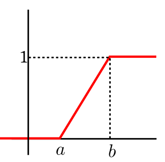
To appreciate the discussion better, you need to recall the following graph from Probability 1:
Distribution function of $Unif(a,b)$
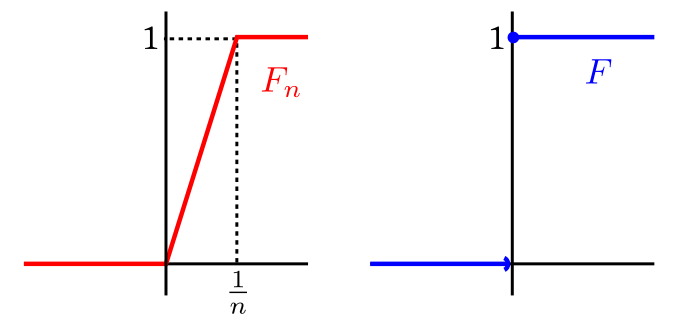
EXAMPLE 3: Suppose that $X_n\sim Unif\left(0,\frac 1n\right).$ Intuitively, what distribution does $(X_n)$ approach?
SOLUTION:
Intuitively the limiting distribution should be degenerate at $0$, i.e., $X_n\rightarrowD X,$ where $X\equiv 0.$
Now let us consider the distribution functions of $X_n$ and $X$:
It might help to see an animation of the convergence of the $F_n$'s:
Notice that we have $F_n(x)\rightarrow F(x)$ whenever $x\neq 0.$ But at $x=0,$ we have $F_n(0)\equiv 0$ while
$F(0) = 1.$ So $F_n(0)\not\rightarrow F(0).$
So to make the mathematics behave intuitively, we need to relax the convergence requirement at the
discontinuity point of
$F.$
■
While convergence in distribution is a natural concept, you should be aware of one pitfall that is illustrated in the next
example.
EXAMPLE 4: Consider a $Unif(0,1)$ probability space, and let $X_n(\omega) = \omega.$ Also
let $X(\omega) = \omega.$ Then obviously $X_n\rightarrowD X$, because they are all actually
the same random variable! But is the following statement also true: $X_n\rightarrowD 1-X$?
SOLUTION:
While it might surprise you, the answer is "Yes!", because $X$ and $1-X$ both have the same distribution, viz.,
$Unif(0,1).$
When we say $X_n\rightarrowD X$, we actually mean
"distribution of $X_n$ $\rightarrow$ distribution of $X$ ".
Since distribution of $X$ is the same as as the distribution of $1-X,$ convergence in distribution does not distinguish
between $X$ and $1-X.$
Indeed, a more reasonable notation is $X_n\rightarrow Unif(0,1).$ Here we are writing the
distribution itself after the arrow, and hence there is no need to use the $\rightarrowD$ notation.
■
Proof:Direct.[QED]
However, we do not have any result like "If $X_n\rightarrowD X$ and $Y_n\rightarrowD Y$, then $X_n\pm Y_n\rightarrowD X\pm Y.$"
The following example explains why.
EXAMPLE 5:
Show that $X_n\rightarrowD X$ and $Y_n\rightarrowD Y$ do not imply $X_n+ Y_n\rightarrowD X+ Y.$
SOLUTION:
We consider a $Unif(0,1)$ probability space. Define $X_n(\omega) = \omega$ and $Y_n(\omega) = \omega.$
Also let $X(\omega) = \omega$ and $Y(\omega) = 1-\omega.$
Then $X_n\rightarrowD X$ and $Y_n\rightarrowD Y.$ But $X+Y\equiv 1,$ while for each $n$ we have $X_n+Y_n \sim Unif(0,2).$
So $X_n+ Y_n\not\rightarrowD X+ Y,$ as required.
■
EXERCISE 24: Let $(a_n)$ be a fixed sequence with $a_n\rightarrow a.$ Let $X_n\equiv a_n$ and
$X\equiv a.$ Then is it true that $X_n\rightarrowD X$?
EXERCISE 25: Let $X_n\sim Bern\left(\frac 1n\right).$ Then show that $X_n$ converge in distribution. Find the limit.
EXERCISE 26: Let $(X_n)$ be a sequence of random variable with distribution function $F_n,$ where
$$F_n(x) = \left\{\begin{array}{ll}0&\text{if }x < 0\\ x^n&\text{if }x\in[0,1)\\ 1&\text{otherwise.}\end{array}\right.. $$
Show that $X_n\rightarrowD X$ for some $X.$ What is the distribution of $X$?
EXERCISE 28: If $X_n\sim Unif\left(\frac{\sqrt n-\sqrt 2}{2\sqrt n},\frac{\sqrt n+\sqrt 2}{2\sqrt n}\right),$
then does $(X_n)$ converge in distribution? If so, find the limiting distribution.
EXERCISE 29: If $X_n\sim Unif\left(n-\frac 1n,n+\frac 1n\right),$
then does $(X_n)$ converge in distribution? If so, find the limiting distribution.
EXERCISE 30: Let $U_1,...,U_n$ be iid $Unif(0,1)$ random variables. Let $X_n = \min_i U_i.$ Show that $X_n\rightarrowD 0.$
Hint:
Distribution function of $X_n$ is $F_n(x) = P(X_n\leq x) = 1-P(X_n > x) = 1-P(\forall i~~U_i > x).$
EXERCISE 31: $(X_n), X$ are discrete random variables taking values in $\{1,...,10\}.$ If pmf
of $X_n$ converges pointwise
to pmf of $X,$ then show that $X_n\rightarrowD X.$
The Central imit Theorem (CLT) is possibly the most famous theorem in probability theory and statistics. Originally stated
and proved by Gauss, the theorem has many variants due to other mathematicians. Here we shall state the simplest version.
Proof:Skipped.[QED]
This theorem is a manifestation of statistical regularity. Whatever may the true
distribution of the $X_i$'s be, if you average a large number of $X_i$'s you get a close
approximation to the normal distribution. This allows
statistician to deal with averages of a large number of IID observations without knowing the true
underlying distribution.
Let's look at a typical example.
EXAMPLE 6: If 40% of the population of a city supports a poll candidate, then what is the approximate
probability that a random sample of 500 persons from the city will have at least 250 supporters?
SOLUTION:
Here we think of the sampling procedure as 500 trials of the same random experiment: Pick a person at random
from the population of the city.
We shall assume that the trials are iid.
Actually the trials are neither independent nor identially distributed,
because we typically
sample
without replacement in such a scenario. So the first
member of the sample was drawn from the entire population, while
the second member was drawn from the rest of the
population.
However, since the population is large (much
larger than 500), so we are ignoring both the non-identical and dependent nature and assuming iid.
Our random variable is:
$$X(\omega) = \left\{\begin{array}{ll}1 &\text{if }\omega\mbox{ supports the candiate}\\ 0&\text{otherwise.}\end{array}\right.$$
Here $\omega$ is the person sampled. Each trial gives rise to one copy of this random variable, so we have
$X_1,...,X_{500}$ iid $Bernoulli(0.4).$ This $0.4$ came from the 40% given in the problem.
By CLT we have
$$\frac{\sqrt n (\bar X_n-\mu)}{\sigma}\rightarrow N(0,1)$$
as $n\rightarrow \infty,$ where $\mu = E(X_i)$ and $\sigma^2 = V(X_i)< \infty.$ We shall write this as
$$\bar X_n \stackrel{\bullet}{\sim} N\left(\mu,\frac{\sigma^2}{n}\right)$$
for large $n.$ Here $\stackrel\bullet\sim$ means "approximately distributed as".
In our case, $\mu = 0.40$, $\sigma^2 = 0.4(1-0.4) = 0.24$ and $n=500.$ So
$$\bar X_{500} \stackrel{\bullet}{\sim} N\left(0.40,\frac{0.24}{500}\right),$$
or
$$\sum_1^{500} X_i \stackrel{\bullet}{\sim} N(0.40\times 500,0.24\times 500)\equiv N(200, 120).$$
Now we can find the required probability as
$$P(\sum_1^{500} X_i \geq 250) \approx 1-\Phi\left(\frac{250-200}{\sqrt{120}}\right).$$
This probability may be obtained by looking up standard $N(0,1)$ tables or using R as
1-pnorm((250-200)/sqrt(120))
■
In this problem we knew the distribution of the $X_i$'s, but we never really made any use of it, except to compute $E(X_i)$
and $V(X_i).$
We have learned about four different modes of convergence. It is surprising
and somewhat disconcerting that these modes are not equivalent. The following diagram shows the relative strengths of the
these modes.
Whenever there is a blue arrow from one mode to another, the first mode implies the second mode.
None of the other implications hold in general.
Here we shall use the fact that if for a sequence of events $(A_n)$ we have $P(A_n\io)=0$ then $P(A_n)\rightarrow 0.$
We had seen this in the Borel-Cantelli page.
Proof:
To show $\forall \epsilon>0~~P(|X_n-X|\geq \epsilon) \rightarrow 0$ as $n\rightarrow \infty.$
Take any $\epsilon>0.$
Let $A_n = \{|X_n-X|\geq \epsilon\}$.
Since $X_n\rightarrowA X,$ hence
$P(A_n\io) = 0.$
Hence $P(A_n)\rightarrow 0.$
[QED]
Since $L_1$ is the weakest member of the $L_p$ family (for $p\geq 1$), we shall
take $L_1$ as the representative of $L_p$ in the following discussion.
Proof:
Take any $\epsilon>0.$ Then, by Markov inequality applied to $|X_n-X|$ (which is
nonnegative thanks to the modulus), we have
$$P(|X_n-X|>\epsilon)\leq \frac{E(|X_n-X|)}{\epsilon}\rightarrow 0.$$
[QED]
Though convergence in distribution does not imply convergence in probability in general, but there is one important special
ase where it does! This is given in the theorem below.
Proof:
Since $X_n\rightarrowD C,$ hence $\forall x < c~~P(X_n\leq x)\rightarrow 0$ and $\forall x \geq c~~P(X_n\leq x)\rightarrow 1$
Shall show $X_n\rightarrowP c,$ i.e., $\forall \epsilon>0~~P(|X_n-c| > \epsilon)\rightarrow 0.$
Take any $\epsilon>0.$
Then
$$\begin{eqnarray*}
P(|X_n-c| > \epsilon) & = & P(X_n < c-\epsilon \mbox{ or } X_n > c+ \epsilon)\\
& = & P(X_n < c-\epsilon)+P(X_n > c+ \epsilon)\\
& = & P(X_n < c-\epsilon)+1-P(X_n \leq c+ \epsilon)\\
& \leq & P(X_n < c-\epsilon)+1-P(X_n \leq c+ \epsilon)\\
& \rightarrow & 0 + 1-1 = 0.
\end{eqnarray*}$$
Hence, by sandwich law of limit, $P(|X_n-c| > \epsilon\rightarrow 0,$ as required.[QED]
The following example shows that almost sure convergence does not imply $L_p$ convergence, even when the $p$-th
moments exist finitely for all the random variables involved.
EXAMPLE 7: We work with $Unif(0,1)$ probability space. Let $X_n(\omega) = \left\{\begin{array}{ll}n&\text{if }\omega\in\left(0,\frac 1n\right)\\ 0&\text{otherwise.}\end{array}\right.$.
Let $X\equiv 0.$
Then clearly $\forall\omega\in (0,1)~~X_n(\omega)\rightarrow X(\omega).$ Hence $X_n \rightarrowA X.$
But $\forall n\in{\mathbb N}~~E(X_n) = n\times\frac 1n = 1\not\rightarrow 0 = E(X).$
■
Other counterexamples are in the problem set below.
EXERCISE 35: Let $f_1,f_2,f_3,...:[0,1]\rightarrow{\mathbb R}$ be defined as indicator functions of
$[0,1],$
$\left[0, \frac 12 \right], \left[ \frac 12, 1 \right], $
$\left[0,\frac 13 \right], \left[ \frac 13, \frac 23 \right], \left[ \frac 23, 1 \right], $
etc. Let $U\sim Unif[0,1].$ Let $X_n = f_n(U).$ Let $X\equiv 0.$ Show that
$X_n\rightarrowL 1 X$ but $X_n\not\rightarrowA X.$
EXERCISE 36: Consider $X_n, X$ as in the last exercise. Show that $X_n\rightarrowP X.$
EXERCISE 37: Among the examples discussed so far, there is one counterexample that shows that
convergence is probability does not imply $L_1$ counterexample. What is that example?
Convergence in distribution obviously cannot imply convergence in probability, because
convergence in distribution does not even require the random variables to be defined on the same
probability space. But even if all the random variables are defined on a common probability
space, we can get a counterexample, as shown in the next problem.
EXERCISE 38:
Let $U\sim Unif(0,1).$ Let $X_n = (-1)^n U.$ Then
show that $X_n\rightarrowD U,$ but $X_n\not\rightarrowP U.$