[Home]
Table of contents
$
\newcommand{\v}{\vec}
$
Differential equations
| Last
updated on:
SUN JAN 24 IST 2021 |
During our high school days we are taught that a simple pendulum executes an
approximately simple harmonic motion if the angle of swing is small. However, high
school textbooks avoid discussing the general case: the motion of a
pendulum that may swing to larger angles. The main reason is that this leads
to an unmanageable differential equation that cannot be solved without a computer.
Consider the following diagram.
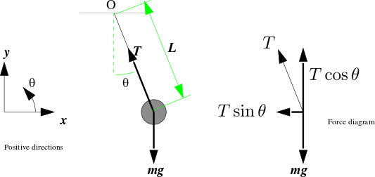 |
| Simple pendulum |
Taking $O$ as the origin and positive
$x$- $y$- and $\theta$-directions as shown, the position of
the bob is
$$\begin{eqnarray*}
x & = & L\sin(\theta)\\
y & = & -L\cos(\theta).
\end{eqnarray*}$$
Remember that $\theta $ is a function of time $t.$ So the above
equations actually mean
$$\begin{eqnarray*}
x(t) & = & L\sin(\theta(t))\\
y(t) & = & -L\cos(\theta(t)).
\end{eqnarray*}$$
The forces on the bob along the positive $x$- and $y$-directions
are, respectively,
$$\begin{eqnarray*}
F_x & = & -T\sin(\theta)\\
F_y & = & T\cos(\theta)-mg.
\end{eqnarray*}$$
Here $T$ is the tension in the rod. It is also a function of
$t.$
To derive the equations of motion we shall use Newton's second law of
motion, which says
$$\begin{eqnarray*}
F_x & = & m x''\\
F_y & = & m y'',
\end{eqnarray*}$$
where $x''$, $y''$ denote the second derivatives of $x(t)$, $y(t)$ with respect
to $t.$
Differentiating $x(t)$ and $y(t)$ twice we get
$$\begin{eqnarray*}
x'' & = & -L \sin(\theta)(\theta')^2 + L \cos(\theta)\theta ''\\
y'' & = & L \cos(\theta)(\theta')^2 + L \sin(\theta)\theta ''.
\end{eqnarray*}$$
Putting these in Newton's second law, and simplifying, we get
$$
\theta '' = -\frac gL \sin(\theta).
$$
At this point most textbooks use
the ``$\sin(\theta)\approx \theta $'' approximation for "small"
$\theta$ to reduce the above differential equation to
$$
\theta '' = -\frac gL \theta,
$$
which can be solved easily by hand to produce simple harmonic
motion. The approximation is pretty good if the pendulum swings
within $4^\circ$. But not all pendulums swing within that
range. What if you have a pendulum that swings $30^\circ?$
That's what we are going to explore now.
We first reduce the second
order differential equation $\theta '' = -\frac gL\theta$
to a system of first order equations.
$$\begin{eqnarray*}
\theta ' & = & \omega\\
\omega' & = & -\frac gL \theta.
\end{eqnarray*}$$
Notice that $(\theta',\omega')$ is given as a function
of $(\theta,\omega).$ The entire motion of the pendulum is
determined if we know $(\theta,\omega)$ at some instant. So
we call $(\theta,\omega)$ the phase of the system. We
are given the initial phase of the system, i.e., we know from which initial angle we have released the
pendulum, and with what angular velocity. Our aim is to know the phase at
all time points during the swing.
Thus, at $t=t_0$ (specified number), we know
$$\begin{eqnarray*}
\theta & = & \theta_0\mbox{ (specified number)},\\
\omega & = & \omega_0\mbox{ (specified number)}.
\end{eqnarray*}$$
We want to know the values $\theta(t)$ and $\omega(t)$ at any given $t > t_0.$
Thanks to the differential equations, we also know
the rate at which they are increasing at $t=t_0:$
$$\begin{eqnarray*}
\theta'(t_0) & = & \omega_0,\\
\omega'(t_0) & = & -\frac gL\sin \theta_0.
\end{eqnarray*}$$
Now advance time a little to $t_1=t_0+\delta t$, say. By this
time $\theta$ and $\omega$ will roughly change to
$$\begin{eqnarray*}
\theta_1 & = & \theta_0 + \theta'(t_0)\delta t = \theta_0+\omega_0\delta t\\
\omega_1 & = & \omega_0 +\omega'(t_0)\delta t =
\omega_0-\frac gL\sin \theta_0 \delta t.
\end{eqnarray*}$$
So we get the phase (approximately) at $t_1= t_0+\delta t.$
Now we keep on advancing time by $\delta t$ increments. The same
logic may be used repeatedly to give, at $t_k = t_0+k\cdot\delta t,$
$$\begin{eqnarray*}
\theta_k & = & \theta_{k-1} + \omega_{k-1}\delta t\\
\omega_k & = & \omega_{k-1} -\frac gL\sin \theta_{k-1} \delta t.
\end{eqnarray*}$$
Admittedly, this is a rather crude approximation. However, if $\delta t$ is pretty small, the accuracy increases.
Let us explore this numerically using J. For this, consider the
iteration as a single function that maps one $(\theta,
\omega)$ pair to the next:
$$
(\theta,\omega)\mapsto (\theta,\omega) + \delta t
\underbrace{\left(\omega,-\tfrac gL\sin \theta\right)}_{r(\theta,\omega),\mbox{ say}}.
$$
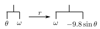
r=: {:, (_9.8 * sin @ {.)
Rememebr that this function is expeced to work as a monad on a
pair $(\theta,\omega).$ Notice that the J code is
essentially the same as the following description
of $r(\theta,\omega)=\left(\omega,-\tfrac gL\sin \theta\right)$ in plain English:
the last entry (i.e., $\omega$) followed
by $-9.8\times$ the first entry (i.e., $\theta $).
Next, have to move from the current $r(\theta,\omega)$ pair
to the next.
English description:
Add $\delta t\times r$ (to the current value).
Its J translation gives a function u:
u=: + 0.1 * r
Try out r and u like this with initial $(\theta,\omega)=(1,0)$:
r 1 0
u 1 0
Since J codes are minimalistic, it is easy to lose your
bearing while programming. To avoid this, keep a firm hold on
the layout of the data as they get transformed by
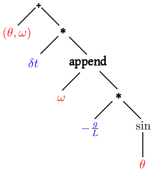
different functions. For instance, the updating function
produces the next $(\theta,\omega)$ pair from the current one:
this:
It will help to visualize the updation as a syntax tree:
It should not be very difficult to draw (mentally, after some
practice) this tree based on the algebraic description. The only
hitch may be with the "append" function which is something we are
not as familiar as the mathematical operations. This is more like
a book-keeping operation, but thanks to J's infix notation we can
show this in the same syntax tree as the more mathematical
ones.
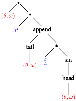
In a syntax tree, the data enter through the leaves. There
are two types of data here: those involving the current value
(shown in red) and those involving various constants
(shown in blue). Our plan is to express this as a function
of $(\theta,\omega)$. So we need two book keeping functions
to extract $\theta $ and $\omega$
from $(\theta,\omega),$ resulting in the following tree:
This syntax tree may be written down directly in J:
u=: + 0.1 * {: , _9.8 * sin @ {.
This may look like a magic spell (it is one!), but if you wish,
you may resort to a more verbose version:
r=: {: , _9.8 * sin @ {.
u=: + 0.1 * r
Let us compare this with a similar thing from, say, Python:
r = [ y[1], -9.8 * sin(y[0]) ]
y = y + 0.1 * r
If you want to start with some y and apply this 10 times,
then you will need to replay both the lines as many
times. But in J, r is a function, and it is already
inside u. So merely applying u 10 times will be
enough. Let us see this in action.
We shall start with initial $(\theta,\omega)=(1,0)$ and
apply the function updating function 100 times, say.
u^:(i.100) 1 0
Here we are using the function power operator. If u is a
function then u ^: 2 will apply it twice
(i.e., $y\mapsto u(u(y))$). If we write u ^: 1 2 3,
then you will get a function ($f$, say) such
that $f(y)$ is a tree with items $u(y)$, $u(u(y))$
and $u(u(u(y))).$
Here i.100 is the list $0,1,2,...,99.$ So we are
getting 99 iterations of the function u starting with $(\theta,\omega)=(1,0)$.
This is what you get:
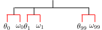
It will be a lot more fun to make a plot of the $\theta$
values. To isolate just the $\theta$ values, you need to
pick up only the first entry (i.e. apply {.) to each of
the red subtrees (i.e., at rank 1):
plot {."1 u^:(i.100) 1 0
J help
-
=: defining a new variable or function.
-
{. (head): extracts the first element of a list.
-
{: (tail): extracts the last element of a
list.
-
@ function composition.
-
^: (composition power): e.g. f^:3
means $f(f(f(\cdots))).$ Also, f^:(1 2 3)
means a list of functions, $f, f\circ f, f\circ f\circ f.$
-
i. creates a list of integers. In particular,
i. 5 is 0,1,2,3,4.
-
|: (transpose): matrix transposition.
-
plot when used as plot y makes a
line plot of $(0,y_0),...,(n-1,y_{n-1})$ if $n$ is the
length of $y.$
Our differential equation was of the form
$$y'(t) = f(y),$$
where $y(t_0) = y_0.$ In our pendulum example we had $y
= (\theta,\omega).$ Also
$$
f(y) \equiv f(\theta, \omega) = \left(\omega, -\frac gL\sin \theta\right).
$$
The crude approximation that we used is called Euler's
method. It works with the more general form:
$$
y'(t) = f(t,y),\quad y(t_0) = y_0.
$$
We shall be given the function
$f(\cdot,\cdot)$ and the initial values $t_0,y_0.$ We are also given a
positive integer $n$ and a step size $\delta t.$ We have to find out the
function $y(t)$ at the points $t_1,...,t_n,$ where
$$
t_i = t_0+i \delta t.
$$
Euler's method works by making local linear
approximations to the unknown $y(t).$
For this we need to know the derivative of $y(t).$ If
at some instant $t$ we can guess the value of $y(t),$ then the value of $y'(t)$ may be obtained from
differential equation: $y'(t)=f(t,y(t)).$
Here we are starting from $y_0 =
y(t_0).$ So we know that $y'(t_0) = f(t_0,y_0).$ This is the slope
of the tangent to $y(t)$ at $t=t_0.$ Follow this tangent for
a little time $\delta t$ to arrive at $y_1 =
y_0+f(t_0,y_0)\delta t.$ The point
$(t_1,y_1)$ may not lie exactly on the curve of $y(t).$ But if $\delta t$
is small, then this should lie close to it. So we take $y_1$ as an
approximation to $y(t_1).$ Now we repeat the process again to get
$y_2 = y_1+\delta t\,f(t_1,y_1).$ In general, we define
$$
y_k = y_{k-1}+\delta t\, f(t_{k-1},y_{k-1}) \quad\mbox{ for } k=1,...,n.
$$
This is Euler's method.
How good is this method? To explore this we shall try out a simple example, where
the solution is known.
EXAMPLE:
Suppose we are working with $f(t,y) = -\sin(t+y).$ In other
words, we are solving $\frac{dy}{dt} = -\sin(t+y).$ We shall
start from the point $\left(0,-\frac \pi2\right),$ i.e., $y = -\frac \pi2$
when $t=0.$
Of course,
we can solve it analytically, by taking $v = t+y.$
Then $\frac{dv}{dt} = 1+\frac{dy}{dt}= 1-\sin(v),$ which may be solved by direct integration. The
answer is (check!)
$$
y = -\sin ^{-1} \left( \frac{1-t^2}{1+t^2} \right) - t.
$$
We
shall compare our approximation with this to
see how Euler's method performs. We shall take $n$ steps
in $[0,2].$ Then the Euler iterations are
$$
y_i = y_{i-1} - \frac 2n\times \sin(t_{i-1}+y_{i-1})
$$
for $i=1,...,n$ starting with $t_0 = 0$ and $y_0 =-\frac \pi2.$
The result (with $n=10$) is shown in the following graph. The continuous curve is the true solution. The dashed
polyline (with 10 segments) is Euler's approximation:
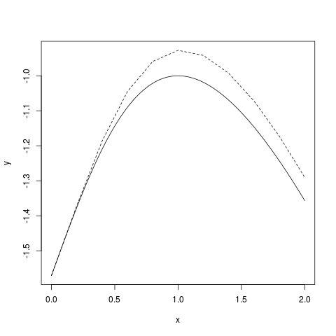 |
| Euler with 10 steps |
If we increase the number of steps to 20 then the approximation
is somewhat better:
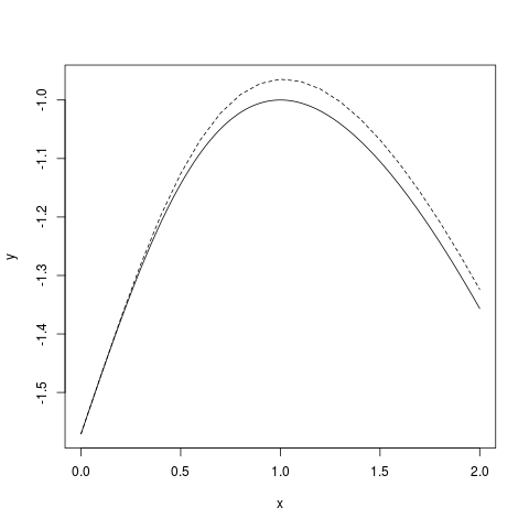 |
| Euler with 20 steps |
If you use 100 steps the accuracy is pretty good:
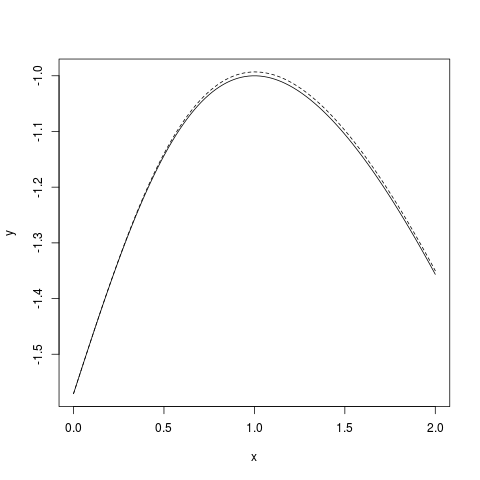 |
| Euler with 100 steps |
We may explore these using the following J code.
d1=:-@sin@+/
eu=:] + 0.1, 0.1  *  d1
eu^:(i.5) 0 _0.5p1
xct=: --arcsin@ (1 (-%+) *~)
tr=: xct t=: (i.200) % 100
pd'reset'
pd t; tr
pd ;/ |: eu^:(i.20) 0 _0.5p1
pd'show'
J help
-
+/ means summation. e.g. +/ 1 2 3
will give 6.
-
, joins two lists end to end. e.g. if $x=1, 2,
3$ then 5, x means 5,1,2,3.
-
_0.5p1 means $-\frac \pi2.$
-
(f g h) means the function $y\mapsto
g(f(y), h(y)),$ or $(x,y)\mapsto g(f(x,y), h(x,y)).$ Just as $(\sin+\cos)(x) = \sin x + \cos
x.$ In particular, 1 (-%+) x means $\frac{1-x}{1+x}.$
 Now try your hand at the following problem.
EXERCISE:
$\frac{dy}{dx} = e^{-xy^2}$ starting from $(0,0).$
One problem with Euler's method is that unless $\delta t$ is very small the
$y_i$'s may move away from the curve of $y(t).$ Taylor's
method generalises Euler's method to improve the accuracy. In Euler's
method we used local linear approximations (tangents)
to $y(t)$ at each $t_i:$
$$
y(t) \approx y(t_i) + y'(t_i)(t-t_i).
$$
These are just the first two terms of the Taylor expansion
of $y(t):$
$$
y(t_i) + y'(t_i)(t-t_i) + \frac{y''(t_i)}{2}(t-t_i)^2
+\cdots \frac{y^{(k)}(t_i)}{k!} (t-t_i)^k + \cdots
$$
In Taylor's method we take more terms from this series. Thus,
1-st order Taylor's method is the same as Euler's method, while
the $k$-th order Taylor's method uses
$$
y(t)\approx y(t_i) + y'(t_i)(t-t_i) + \frac{y''(t_i)}{2}(t-t_i)^2
+\cdots \frac{y^{(k)}(t_i)}{k!} (t-t_i)^k.
$$
EXERCISE: Check that it is the unique $\leq k$ degree polynomial that has the same
derivatives as $y(t)$ up to order $k$ at $t_i.$
EXAMPLE: Solve the same differential equation
$y'(t) = -\sin(t+y)$ with $y(0) = -\frac \pi2$
over $[0,2]$
using 2-nd order Taylor method.
SOLUTION:
The 2-nd degree Taylor polynomial for $y(t)$ at
any $t_{k-1}$ is
$$
y(t_{k-1}) + y'(t_{k-1})(t-t_{k-1}) + \frac{y''(t_{k-1})}{2} (t-t_{k-1})^2.
$$
For this we need $y'(t_{k-1})$ and $y''(t_{k-1}).$ These may be obtained approximately as follows.
We can write the differential equation as
$$
y'(t) = -\sin(t+y(t)).
$$
Differentiating w.r.t. $t,$
$$
y''(t) = -\cos(t+y(t))(1+y'(t)).
$$
Hence
$$\begin{eqnarray*}
y'(t_{k-1}) & = & -\sin(t_{k-1}+y(t_{k-1}))\\
y''(t_{k-1}) & = & -\cos(t_{k-1}+y(t_{k-1}))(1+y'(t_{k-1})).
\end{eqnarray*}$$
As before we take a grid of values in $[0,2],$ say $10$ steps. So
there are 11 points starting with $t_0=1$ and ending
with $t_{10}=2.$ The general formula for $t_k$ is
$$
t_k = 1+k\cdot\delta t,
$$
where $\delta t = \frac 2n.$
So the 2nd order Taylor iterations are
$$y_{k} = y_{k-1} +\frac 2ny'(t_{k-1}) + \frac{2}{n^2}y''(t_{k-1}).$$
The result is shown below. The red curve is the 2nd order Taylor approximation with $n=10.$ The dashed polyline is
the Euler's approximation (i.e., 1st order Taylor) with the same $n.$
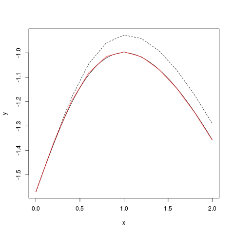 |
| Euler and 2nd order Taylor
($n=10$) |
d1=:-@sin@+/
d2=:(-@cos@+/)*(1+d1)
tay2=:]+0.1, (0.1 * d1) + (0.005 * d2)
tay2^:(i.5) 0 _0.5p1
tr=: xct t=: (i.200) % 100
xct=: --arcsin@ (1 (-%+) *~)
pd'reset'
pd t; tr
pd ;/ |: tay2^:(i.20) 0 _0.5p1
pd'show'
J help
-
; makes boxes, e.g. 1; 'str' ; 3.9
will give a list of boxes.
-
;/ inserts a ; between consecutuve
elements of a list, e.g., ;/ 1 2 3 is the same as 1;2;3.
-
pd makes plots in a versatile way. Start
with pd 'reset' and end with pd
'show'. To plot $(x_i,y_i)$'s and join the points
with line segments use pd x; y