EXAMPLE 1:
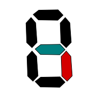
A 7-segment display shows any number from 0 to 9 at random (equal
probabilities).
Let $X$ be the indicator random variable of
whether the blue segment is on. Similarly, $Y$ is the
indicator for the red segment. Find the conditional distribution
of $Y$ given $X.$
SOLUTION:
Here $X,Y$ both take values in $\{0,1\}.$
We need to find $P(Y=y | X=x)$ for $x,y\in\{0,1\}.$
Now $P(Y=1|X=1) = P(X=1,Y=1)/P(X=1).$
Both the blue and the red segments are on in only the numbers
3,4,5,6,8,9. So $P(X=1,Y=1) = \frac{6}{10}.$
The blue segment is on in the numbers 2,3,4,5,6,8,9. So $P(X=1) =\frac{7}{10}.$
Hence $P(Y=1|X=1) = P(X=1,Y=1)/P(X=1) = \frac 67.$
You should now be able to work out the other three conditional
probabilities similarly.
■
We can define conditional CDF or conditional PMF in the obvious
way.
It is important to understand that the conditional
expectation/variance is a random variable, which is a function of
the conditioning random variable.
Arriving at the unconditional distribution from the conditional distribution is easy. There are different ways, all of which
depend on these two facts:
$P(A\cap B) = P(B)P(A|B)$,
the theorem of total probability:
$$
P(A) = P(B) P(A|B) + P(B^c)P(A|B^c),
$$
In both these facts we have expressed unconditional probabilities in terms of conditional ones.
The following two exercises have simple solutions, but are conceptually very important.
::
EXERCISE 1: (Easy)
Let $(X,Y)$ be discrete with $X$ having support $\{x_1,x_2,...,x_m\}$ and $Y$ having support
$\{y_1,y_2,...,y_n\}$.
For $B\subseteq {\mathbb R}$, let $f(x_i, B) = P(Y\in B | X=x_i)$. Then for $A\subseteq {\mathbb R}$ show that
$$P(X\in A,\, Y\in B) = E\big(f(X,B)\ind_{\{X\in A\}}\big).$$
Here $\ind_{\{X\in A\}}$ is the indicator variable for the event $\{X\in A\}$.
The expectation in the RHS is $E\big(f(X,B)\ind_{\{X\in A\}}\big) = \sum_{i:x_i\in A} f(x_i, B)P(X=x_i)$.
What may not be readily obvious is that the converse of the exercise is also true. This is given in
the following exercise.
::
EXERCISE 2: (Easy) Let $(X,Y)$ be as in the last exercise. For $B\subseteq{\mathbb R}$, let $g(x_i, B)$ be such
that for every $A\subseteq {\mathbb R}$ we have
$$P(X\in A,\, Y\in B) = E\big(g(X, B)\ind_{\{X\in A\}}\big).$$
Then show that we must have $g(x_i, B) = P(Y\in B|X=x_i)$ for $B\subseteq{\mathbb R}$ and $i=1,...,m$.
Take $A=\{x_i\}$. [Thanks to Samyak for correcting a typo even in this short answer!]
The above exercise will prove very important later, since it provides a definition of $P(Y\in
B|X=x_i)$ free of explicit division by $P(X=x_i)$. This freedom will later allow us to defined conditional distribution
of $Y$ given $X$ when $X$ is continuous.
We can do similar things with conditional
expectation/variance also.
Proof:(For simple $X,Y$):
Let $X$ take values $x_1,x_2,...,x_m$ and $Y$ take
values $y_1,y_2,...,y_m$. Let the joint PMF of $(X,Y)$ be
$$
P(X=x_i~\&~Y=y_j) = p_{ij}.
$$
Then $P(Y=y_j | X=x_i) = \frac{p_{ij}}{p_{i\bullet}}.$
So $E(Y|X=x_i) = \sum_j y_j \frac{p_{ij}}{p_{i\bullet}}.$
Expectation of this is
$$
\sum_i E(Y|X=x_i) p_{i\bullet} = \sum_i \sum_j y_j
\frac{p_{ij}}{p_{i\bullet}}p_{i\bullet} = \sum_i \sum_j y_j p_{ij} =
\sum_j y_j \sum_i p_{ij} = \sum_j y_j p_{\bullet j} = E(Y),
$$
as required.
[QED]
The proof uses little more than rearranginf terms in a sum using associativity and commutativity
of addition. If $(X,Y)$
could take countably infinitely
many values, then also
the same proof would have worked, because all the infinite series involved would have been absolutely
convergent (thanks to the assumption
of finite existence of the expectations involved).
Many expectation problems can be handled step-by-step using this
result. Here are some examples.
EXAMPLE 2:
A casino has two gambling games:
Roll a fair die, and win Rs. $D$ if $D$ is the
outcome.
Roll two fair dice, and win Rs 5 if both show the same
number, but lose Rs 5 otherwise.
You throw a coin with $P(Head)=\frac 13$ and decide to play game
1 if $Head,$ and game 2 if $Tail.$ What is your
expected gain?
SOLUTION:
Let $X$ be your gain (in Rs), and let $Y$ be the outcome of the
toss.
Then $E(X|Y=Head) = 3.5$ and $E(X|Y=Tail) = 5\times\frac{6-30}{36}=-\frac{10}{3}.$
So, by the tower property, $E(X) = E(X|Y=Head)\times P(Y=Head)+E(X|Y=Tail)\times P(Y=Tail) = \cdots.$
[Thanks to Arindrajit for correcting a typo here.]
■
The tower property is very useful for computing expectations
involving a random number of random variables. Here is an
example.
EXAMPLE 3:
A random number $N$ of customers enter a shop in a
day, where $N$ takes values in $\{1,...,100\}$ with
equal probabilities. The $i$-th customer pays a random amount $X_i$,
where $X_i$ takes values in $\{1,2,...,10+i\}$
ith equal probabilities. Assuming that $N,X_1,...,X_N$ are
all independent, find the total expected payments by the
customers on that day.
SOLUTION:
We have $E(X_i) = \frac{11+i}{2}.$
So $E\left(\sum_1^N X_i|N\right) = \sum_1^N E(X_i|N) = \sum_1^N E(X_i) = \sum_1^N \frac{11+i}{2} = 5.5N+\frac{N(N+1)}{4}.$
By tower property, the required answer is $E\left(5.5N+\frac{N(N+1)}{4}\right)=\cdots.$
■
EXAMPLE 4:
10 holes, numbered 1 to 10, in a row. 5 balls are dropped
randomly in them (a hole may contain any number of balls). Call a
ball "lonely" if there is no other ball in its hole or the
adjacent holes. Find the expected number of lonely balls.
SOLUTION:
Define the indicators $I_1,...,I_5$ as
$$
I_i = \left\{\begin{array}{ll}1&\text{if }i\mbox{-th ball is lonely}\\0&\text{otherwise.}\end{array}\right.
$$
Then the total number of lonely balls is $X = \sum I_i.$
So we are to find $E(X) = \sum E(I_i).$
Let $Y_i = $ the hole where the $i$-th ball has fallen.
Then $E(I_i|Y_i=1)$ is the conditional probability that
all the balls except the $i$-th one has landed in
holes $3,...,10$ given that the $i$-th ball has landed
in hole 1.
[Thanks to Nuhad for correcting a typo in the line above.]
You should be able to compute this easily. Similarly, you can
compute $E(I_i|Y_i=k)$ for $k=1,...,10.$
Notice that $Y_i$ can take values $1,...,10$ with equal probabilities.
So tower property should provide the answer as
$$
E(X) = \sum E(E(I_i|Y_i)) = \cdots.
$$
■
Proof:
This follows directly from the tower property.
If $X,Y,Z$ are jointly distributed random variables, then we
can talk about conditional distribution of $Z$
given $(X,Y)$ or $X$ given $Z$ or $(X,Z)$
given $Y,$ etc. We can even condition step by step. For
example, we can talk about $E(E(Z|X,Y)|X).$ This is a
function of $X$ alone.
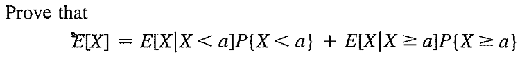
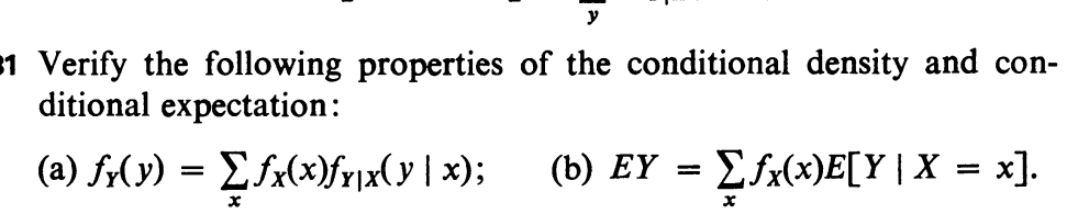
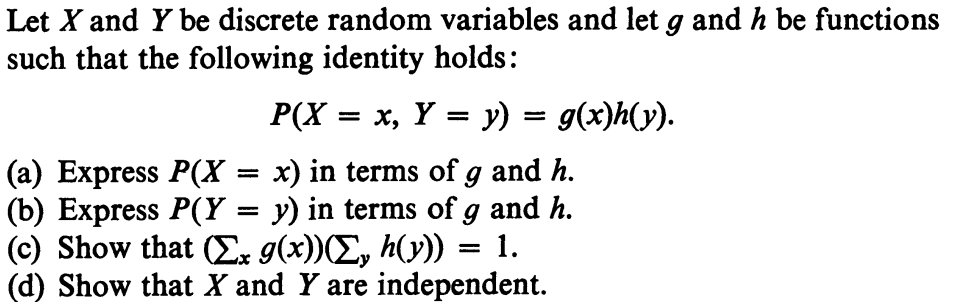
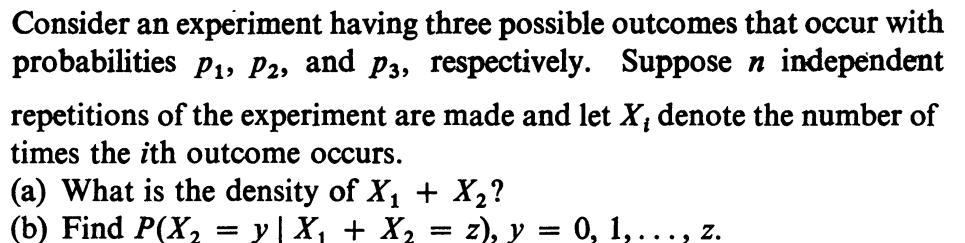
(a) Once you realise that $f_X(x) = P(X=x)$, $f_Y(y) = P(Y=y)$ and
$f_{Y|X}(y|x) = P(Y=y|X=x),$ the given equality is just theorem of total probability.
(b) The RHS is $E(E(Y|X))$ and so the equality is just the tower property.
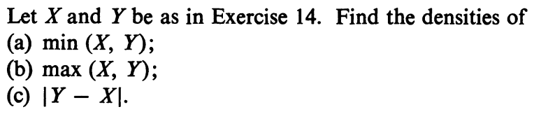
(a) Let $U = \min(X,Y).$ Then $U$ can take values $0,...,N.$
$P(U=k) = P(U\geq k)-P(U\geq k+1).$
Now $P(U\geq k) = P(X,Y\geq k) = P(X\geq k)P(Y\geq k) = \left(\frac{N-k+1}{N+1}\right)^2.$
Similarly, $P(U\geq k+1) = \left(\frac{N-k}{N+1}\right)^2.$
So $P(U=k) = \frac{(N-k)^2-(N-k+1)^2}{(N+1)^2} = ... .$
(b) Let $T = \max(X,Y).$ Then $T$ can take values $0,...,N.$
$P(T=k) = P(U\leq k)-P(T\leq k-1).$
Now $P(T\leq k) = P(X,Y\leq k) = P(X\leq k)P(Y\leq k) = \left(\frac{k+1}{N+1}\right)^2.$
Similarly, $P(T\leq k-1) = \left(\frac{k}{N+1}\right)^2.$
So $P(T=k) = \frac{(k+1)^2-k^2}{(N+1)^2} = \frac{2k+1}{(N+1)^2}.$
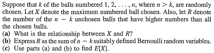
(c) $R=|Y-X|$ can take values in 0,1,...,$N.$
$P(R=0) = P(X=Y) = \frac{1}{N+1}.$
For $k=1,...,N,$ we have $P(R=k) = P(R=k \& X < Y) + P(R=k \& X=Y) + P(R=k \& X > Y).$
Now $P(R=k \& X=Y) =0.$
Also $P(R=k \& X < Y) =P(R=k \& X > Y).$
For $\{R=k\& X < Y\}$ to happen we must have $X = 0,...,N-k$ and correspondingly $Y = k,...,N.$
So $P(R=k\& X < Y) = \frac{N-k+1}{(N+1)^2}.$
Hence $P(R=k) = \frac{2(N-k+1)}{(N+1)^2}.$
[Thanks to Nuhad for correcting a couple of typos here.]
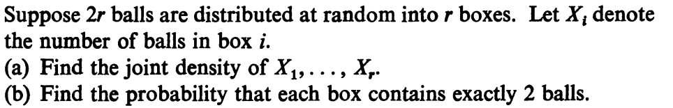
(a) $(X_1,...,X_r)$ can take values $(x_1,...,x_r)$ where each $x_i$ is a nonnegative integer and $\sum_1^r x_i = 2r.$
We consider the random experiment of dropping the balls one by one into the boxes. For each ball have $r $ posible destinations.
So $|\Omega| = r^{2r}.$
Now fix some $(x_1,...,x_r)$ as above. The event $A=\{(X_1,...,X_r) = (x_1,...,x_r)\}$ may be obtained as follows.
Pick and order $x_i$ balls to drop into box $i$ one by one.
So $|A| = \frac{(2r)!}{x_1!\times\cdots\times x_r!}.$
Hence
$P\{(X_1,...,X_r) = (x_1,...,x_r)\}= \frac{ |A| }{ |\Omega| }.$
(b) Let $B$ be the event in question. Then we can compute $|B|$ as follows.
Step 1: Choose two balls to go into box 1: $\binom{2r}{2}$ ways.
Step 2: Choose two other balls to go into box 2: $\binom{2r-2}{2}$ ways.
...
Step 1: Choose the last two balls to go into box r: $1$ way.
So $|B| = \frac{(2r)!}{2^r}$.
Hence $P(B) = \frac{|B|}{|\Omega|} = \frac{(2r)!}{(2r^2)^r}$.
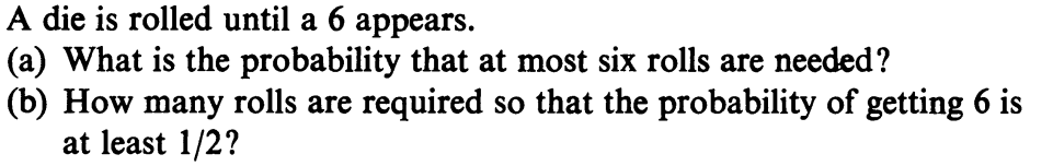
(a) $1-\left(\frac{5}{6}\right)^6.$
(b) For $n$ rolls $P($ at least one 6$)=1-\left(\frac 56\right)^n.$
We need $n$ such that $1-\left(\frac 56\right)^n\geq \frac 12.$
Direct computation shows $n\geq 4.$
::
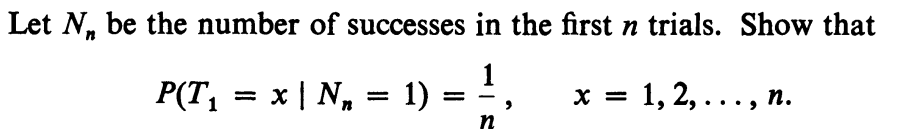
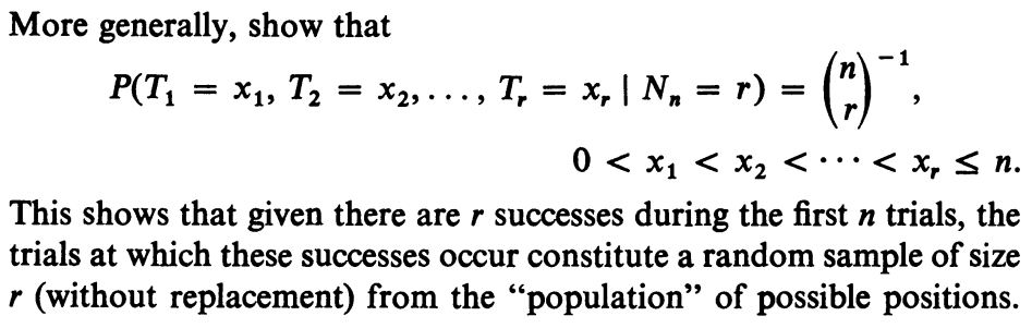
EXERCISE 12: (Medium) [condist10.png]
Imagine this set up: A coin with $P(H)=p$ is repeatedly tossed. Success means $H.$
By symmetry, the answer is $\frac 1n$ if $k=1.$ So, for general $k$ the answer is $\frac kn.$
::
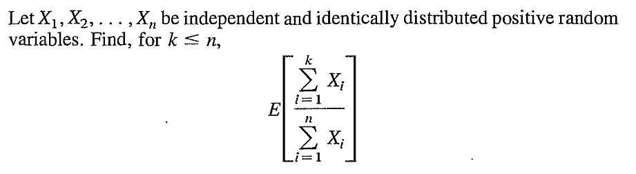
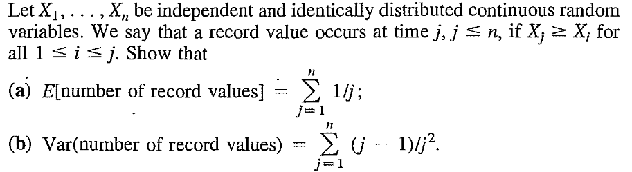
EXERCISE 16: (Hard) [morecond2.png]
Here you should use the fact that for continuous joint distribition $P(X_i=X_j)=0$ for $i\neq j$. Thus, you may
assume that all the $X_j$'s are distinct.
Let $I_j$ be the indicator variable for whether there is a
record at position $j.$ Let $R_j$ be the rank of $X_j$. The smallest of the
$X_j$'s has rank $1$, the largest has rank $n$. Then
$P(I_j=1)$ may be computed
by total probability:
$$
P(I_j=1) = \sum_{k=j}^n P(R_j=k)P(I_j=1|R_j=k).
$$
Similarly for $P(I_jI_k=1).$
[Thanks to Nuhad for pointing out a serious mistake here.]
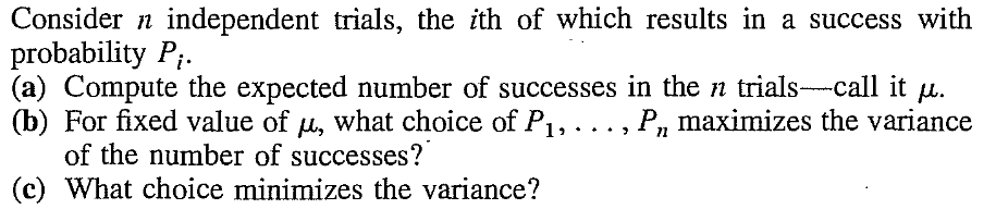
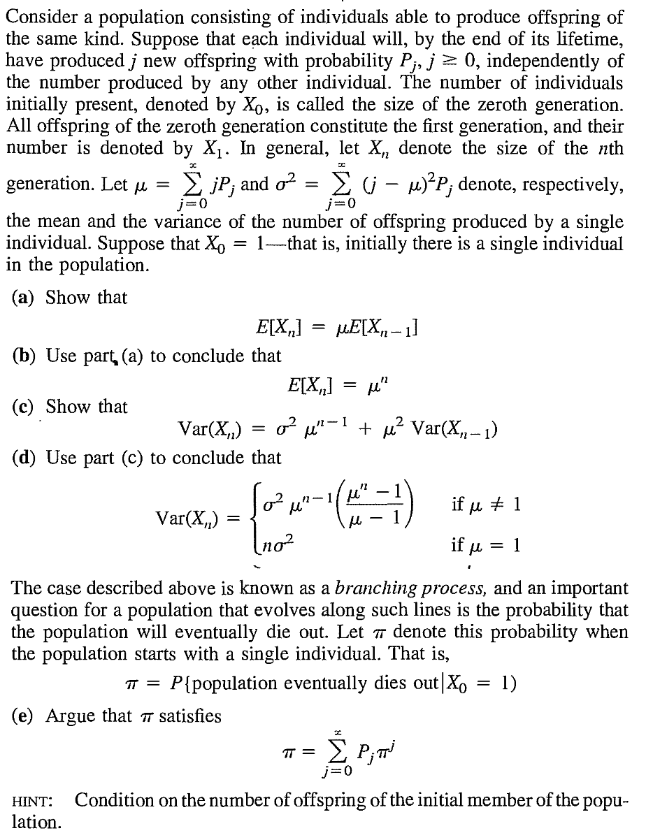
(a) $\mu=\sum P_i$.
(b) The problem is basically minimising $\sum P_i^2$ subject
to $\sum P_i=\mu$ being fixed. Cauchy-Schwarz might help.
(c) Here we have to maximise $\sum P_i^2$ subject to $\sum P_i=\mu.$ First notice that
in any maximising $(P_1,...,P_n)$ all but at most one $P_i$ must be either $0$
or $1$. Because if $P_i,P_j\in(0,1)$ for $i\neq j$, then take the smaller one
closer to zero and the larger one closer to 1 by the same amount. Then $\sum P_i$ remains unaltered, but $\sum P_i^2$
increases.
So the only canidates are where there are exactly $[\mu]$ many $P_i$'s equal to $1$, and (if $\mu$
is not an integer) exactly one $P_i$ equal to $\{\mu\}$, the fractional part of
$\mu$, and the rest equal to 0.
For example, if $n=5$ and $\mu=2.3$, then one candidate is $(1,1,0.3,0,0)$.
Clearly,
for any such candidate the value of $\sum P_i^2$ is the same $([\mu]+\{\mu\}^2)$. Also since we are maximising
a continuous function over a compact set, maximum exists. So these must be the maximising choices.
[Thanks to Samyak for providing the answer to part (c).]
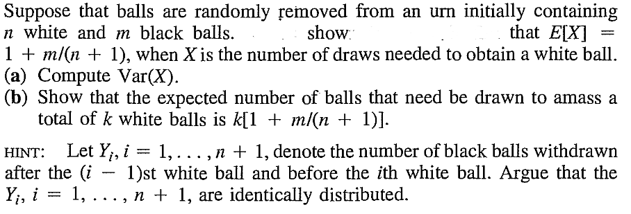
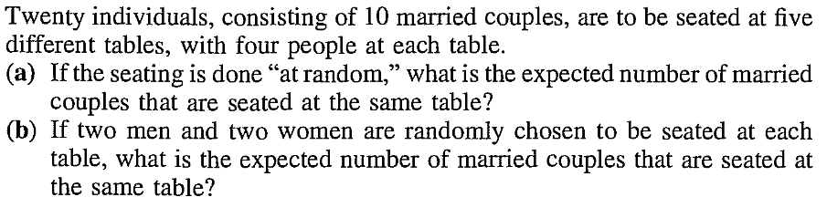
Let the black balls be labelled $b_1,...,b_m.$
Let $X_i=\left\{\begin{array}{ll}1&\text{if }\mbox{no white drawn before }b_i\\
0&\text{otherwise.}\end{array}\right..$
Then $X= 1+\sum_1^m X_i.$
Also, $E(X_i) = \frac{1}{n+1}$. To see this consider the $n$ white balls plus $b_i.$ Out of these $n+1$
balls $b_i$ has the chance $\frac{1}{n+1}$ to come first.
(a) $V(X_i) = \frac{n}{(n+1)^2}.$
Also for $i\neq j$ we have $E(X_iX_j) = \frac{2}{(n+2)(n+1)}$ (because out of the $n$ white balls plus $b_i$
and $b_j$ any of the $\binom{n+2}{2}$ pairs can come first with equal probability).
(b) Let $Y_i$ be as given in the hint. Let's take an example to
understand how $Y_i$'s are defined. Suppose that we have $m=n=2.$
Here is a list of all possible ways these may turn up:
W W B B
W B W B
W B B W
B W B W
B B W W
B W W B
All these are equally likely as the draws are random and do not care about the colours.
Now consider the events $\{Y_1=1\}$ and $\{Y_2=1\}$. These are
$$\{Y_1 = 1\} = \{BWBW, BWWB\}\mbox{ and } \{Y_2 = 1\} = \{WBWB, BWBW\}.$$
As both these have the same size, they also have the same probability. Similarly,
$$\{Y_1 = 0\} = \{WWBB, WBWB, WBBW\}\mbox{ and } \{Y_2 = 0\} = \{WWBB, BWWB, BBWW\}$$
also have the same size, and hence the same probability.
We claim that for any values of $m$ and $n$ and any $i< j$ and any $k$, the events
$\{Y_i=k\}$ and $\{Y_j=k\}$
must have the same size (and hence the same probability).
We show this by demontraiting a bijection $f:\{Y_i=k\}\rightarrow\{Y_j=k\}$ defined as $f(\omega)
= $ the sequence of $W$'s and $B$'s obtained by swapping the $i$-th $W$
and its preceding $B$'s with the $j$-th $W$ and its preceding $B$'s. For
instance, if $m=10, n=5, i=1, j=4, k=2$
then here is an $\omega\in\{Y_i=k\}:$
BBWBWBBWBBBWBBW
Then $f(\omega)$ is
BBBWBWBBWBBWBBW
All swaps are one-one (repeating a swap restores original order). Also $\omega\in\{Y_i=k\}\Leftrightarrow
f(\omega)\in\{Y_j=k\}$. Hence $|\{Y_i=k\}|=|\{Y_j=k\}|$, as required.
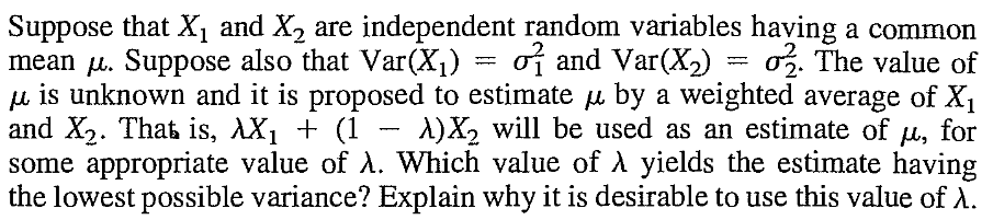
Let $T = \lambda X_1+ (1-\lambda) X_2.$
Then $V(T) = \lambda^2 V(X_1) + (1-\lambda)^2 V(X_2),$ since $X_1,X_2$ are independent.
Thus, $V(T) = \lambda^2 \sigma_1^2 + (1-\lambda)^2 \sigma_2^2 = f(\lambda),$ say.
Then $f'(\lambda) = 2 \sigma^2_1 \lambda - 2 \sigma^2_2(1-\lambda).$
Solving $f'(\lambda) = 0$ we get $\lambda = \frac{\sigma^2_2}{\sigma^2_1+\sigma^2_2}.$
This is desirable because we are giving more weight to the $X_i$ that has less variance (i.e., is more stable).
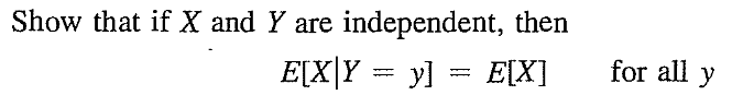
$E(X|Y=y) = \sum_x x P(X=x|Y=y) = \sum_x x P(X=x),$
since $X,Y$ independent.
Hence the result.
::
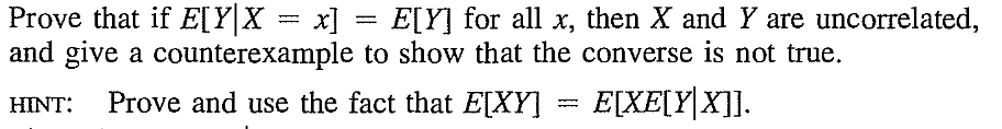
EXERCISE 22: (Easy) [morecond8.png]
Do this for discrete $X, Y$ only. If $X$ can take values $x_1,x_2,x_3,...$ with
positive probabilities, then
you are prove
$$\forall i~~E(g(X)Y|X=x_i] = g(x_i)E(Y|X=x_i).$$
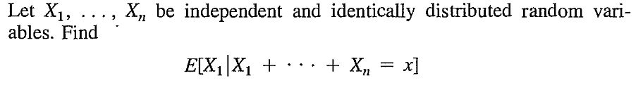
No, the result may not hold if the $X_i$'s have a dependence structure that is
asymetric. A counterexample is as follows.
$X_1 = $ outcome of a roll of a fair die. $X_2$ is obtained from $X_1$ by
swapping 1 and 2. $X_3$ is obtained from $X_1$ by swapping 1 and 3. If the definitions
of $X_2,X_3$ are not clear, then see their values below for all the possible values of $X_1:$
$X_1$
$X_2$
$X_3$
1
2
3
2
1
same as $X_1$
3
same as $X_1$
1
4
same as $X_1$
same as $X_1$
5
same as $X_1$
same as $X_1$
6
same as $X_1$
same as $X_1$
Then
$E(X_1|X_1+X_2+X_3=6)=1\neq \frac 63.$
Here $(X_1,X_2,X_3)$ are jointly distributed with identical marginal distributions. But that does not mean that the
joint distribution of $(X_1,X_2,X_3)$ and $(X_2,X_1,X_3)$ is the same. So in
particular, $E(X_1|X_1+X_2+X_3)$ need not equal $E(X_2|X_1+X_2+X_3)$.
But in the original problem the $X_i$'s were also given to be independent. So there indeed for any permutation $\pi$
of $(1,2,...,n)$ the joint distribution of $(X_1,...,X_n)$ was the same as that of $(X_{\pi(1)},...,X_{\pi(n)})$.
So $E(X_i|X_1+\cdots+X_n)$ was free of $i$.
::
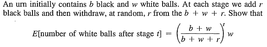
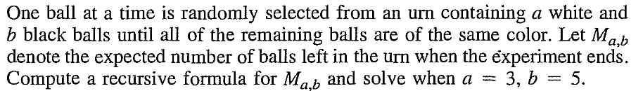
EXERCISE 26: (Medium) [morecond12.png]
Here the random variable of interest is the number of white balls remaining in the urn
after stage $t$. In particular, for $=0$, this numer is $w$.
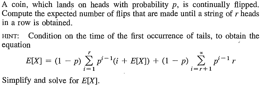
Let's take an example with $r=4$. Consider the tosses until the first tail: $T, HT, HHT, HHHT$ or $HHHH\cdots T$
(i.e., the first tail occurs after toss 4).
Let us encode these cases using a random variable $K$ defined as
$$K = \left\{\begin{array}{ll}i &\text{if }i\mbox{th toss gives first tail and } i\leq 4\\ 5&\text{otherwise.}\end{array}\right.$$
In the last case, $X = 4$.
In the other cases the search starts all over again after the first tail.
So, for $i=1,2,3,4$, we have $E(X|K=i) = i+E(X)$.
Now use tower property.
Let $X$ be the number of balls remaining at the end. Let $Y$ be the indicator variable that the the first selected
ball is white. Then $E(X) = M_{a,b}$ (given) and $E(X|Y=1) = M_{a-1,b}$ and $E(X|Y=0) = M_{a,b-1}$.
Now use tower property to get a recursion.
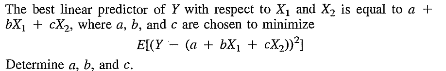
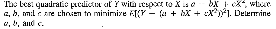
You may expand the expectation as a quadratic expression in $a,b,c$ and partially differentiate it wrt $a,b,c$
and equate to zero to get a set of equations. Then you need to justify that this indeed corresponds to the global minimum.
Or, you may use linear algebra as follows.
Consider the space $span\{1,X_1,X_2\}$. We are trying to find the vector in it that is the closest to $Y$ where
the distance between two random variables $W,Z$ is being measured by $E(W-Z)^2$.
The minimiser must be the foot $\hat Y = a+bX_1+cX_2$ of the perpendicular dropped from
$Y$ onto $span\{1,X_1,X_2\}$.
So we need $Y-\hat Y$ to be orthogonal to $1, X_1$ and $X_2$, i.e., $E(1(Y-\hat Y) = 0$ and $E(X_1(Y-\hat Y) = 0$
and $E(X_2(Y-\hat Y) = 0$. This gives rise to the $3\times 3$ system
$$\left[\begin{array}{ccccccccccc}1 & E(X_1) & E(X_2)\\E(X_1) & E(X_1^2) & E(X_1X_2)\\E(X_2) & E(X_1X_2) & E(X_2^2)
\end{array}\right]\left[\begin{array}{ccccccccccc}a\\b\\c
\end{array}\right] =\left[\begin{array}{ccccccccccc}E(Y)\\E(X_1Y)\\E(X_2Y)
\end{array}\right].$$
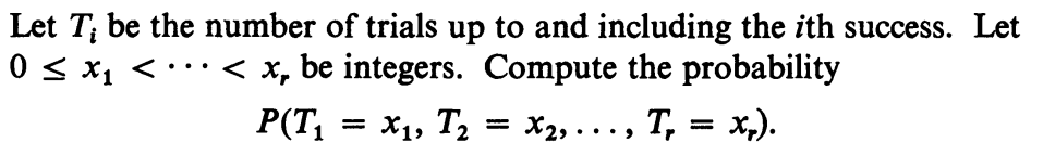
Condition on the number of times you have rolled the die. If you have rolled it $k$ times, then the $k$-th outcome
could not have occured earlier also.
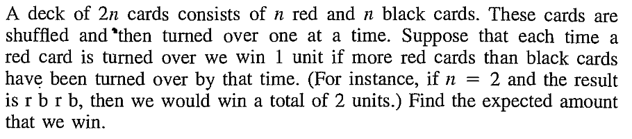
Let $X_i$ be the indicator for $i$-th red ball being a win.
There are $\binom{2n}{n}$ sequences of $n$ R's and $n$ B's in all. Let us count
how many of these lead to $\{X_i=1\}.$
Split each such sequence into two parts, the part before the $i$-th R, and the part after.
For instance, for $n=4$ and $i=3$ the sequence RRBRBRBB is split as RRBRBRBB.
For general $n$ and $i,$ the red part must consist of exactly $i-1$ R's and at
most $i-1$ B's. The blue part consists of exactly $n-i$ R's and the remaining B's.
Let $N_{r,b} = $ number of sequences with exactly $r$ R's and $b$ B's. In other words, $N_{r,b} =\binom{r+b}{r} = \binom{r+b}{b}. $
Then, for any sequence in $\{X_i=1\}$ the red part may be selected in
$$\sum_{j=0}^{i-1} \binom{i+j-1}{j}$$
ways. Here $j$ denotes the number of B's in the red part. Once we also count the matching number
of blue parts for each value of $j$, we get the size of $\{X_i=1\}$ as
$$\sum_{j=0}^{i-1} \binom{i+j-1}{j}\binom{2n-i-j}{n-j}.$$
Quite mysteriously (to me), this is free of $i$ and indeed equals $\frac 12\binom{2n}{n}$.
[Thanks to Souradip for observing this.]
So we see that $P(X_i=1) = \frac 12$. In other words, all the $X_i$'s are actually
identically distributed. (There must be a direct intuitive proof of this, but it beats me!).
So the final answer is just $\frac n2$.
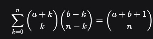
[Souradip found this identity from the web which immediately leads to the mysterious result:
But I do not know an intuitive proof of this identity either!]
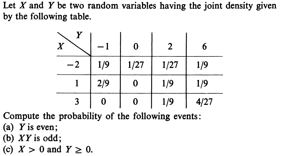
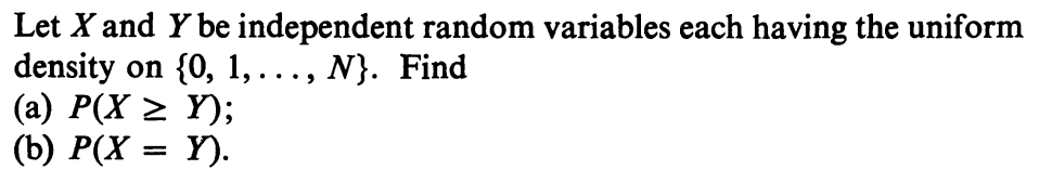
 Here "density" means "PMF".
 Here you should use the fact that for continuous joint distribition $P(X_i=X_j)=0$ for $i\neq j$. Thus, you may
assume that all the $X_j$'s are distinct.
Here you should use the fact that for continuous joint distribition $P(X_i=X_j)=0$ for $i\neq j$. Thus, you may
assume that all the $X_j$'s are distinct.