Notation:Geom$(\theta),$ where $0 < \theta <1.$
Sample space: {1,2,3,...}.
PMF:
$$
P(X=x) = \left\{\begin{array}{ll}
(1-\theta)^{x-1}\theta &\text{if }x=1,2,3,...\\
0 &\text{otherwise.}
\end{array}\right.
$$
Terminology: Such an $X$ is said to have (or follow) Geom$(\theta)$
distribution. We also say that $X$ is a Geom$(\theta)$ random
variable, and write $X\sim$Geom$(\theta).$
Some people (including those who created the R software)
use a slightly different convention. For them the number
of '$0$'s preceding the first '$1$' is a Geometric
random variable.
barplot(dgeom(0:10, prob=0.5))
In R each distribution has a short name. It is geom
for the Geometric distribution. For each distribution there are 4
functions in R: these are formed by appending the
prefixes d, p, q
and r before the short name. The d
prefix gives the PMF, e.g., dgeom. The
prefix p gives the CDF,
e.g., pgeom. The prefix q gives the
"inverse" of the CDF, also called the quantile
function. Finally, the r prefix generates random
number from the distribution.
data = rgeom(1000, prob=0.5)
table(data)
barplot(table(data))
Where used: Suppose that we have a Bern$(\theta)$
random experiment. Let us perform the experiment again and again
independently until we obtain the first `1'. Then count the total
number of
experiments you have done (among these all but the last one have produced
outcome `0'.) The total number of experiments performed is a random
variable with Geom$(\theta)$ distribution.
Let us derive the PMF using the above description. Suppose that we
have a coin with $P(head)=\theta.$ We keep on tossing it until we get
the first head. Suppose that the first head comes at the $x$-th
toss. Then the first $x-1$ tosses are all tails:
$$
\underbrace{TT\cdots TT}_{x-1}H
$$
Each of these tails occurs with probability $(1-\theta)$ and the
final head occurs with probability $\theta.$ So the
probability of
having the first head at the $x$-th toss is
$$
\underbrace{(1-\theta)\times\cdots\times(1-\theta)}_{x-1}\times \theta
= (1-\theta)^{x-1} \theta,
$$
which is the Geom$(\theta)$ PMF
You will need the geometric series here.
$$\begin{eqnarray*}P(X\mbox{ is even})&=& P(X=2)+P(X=4)+\cdots\\
&=&(1-\theta)\theta +(1-\theta)^3 \theta+
(1-\theta)^5 \theta+\cdots\\
&=& \theta(1-\theta)\left[
1+(1-\theta)^2 + (1-\theta)^4+\cdots\right].
\end{eqnarray*}$$
The answer is $\frac{1-\theta}{2-\theta}.$
EXAMPLE 2:
Some versions of Ludo require you to get a `6' on the die before your
counter can move. Sometimes it takes frustratingly long time before you
finally roll a `6'. Let $X$ denote the number of rolls required to
get the first `6'. If we assume the die is fair (i.e., each side has
probability 1/6 of turning up), then what is the distribution of $X?$
SOLUTION: $X$ is a Geom(1/6) random variable.
■
::
EXERCISE 3: (Easy)
In the above example compute the probability of getting the first `6' within
the first 3 rolls.
EXERCISE 4: (Easy)
Some couples are so keen about having a son that they go on producing
babies until they get their first son, and then they stop having children.
Assume that at each birth a baby of
either gender is equally likely. Also assume that the births are
independent. Compute the probability that such a couple has exactly 2
daughters.
EXAMPLE 3:
When a computer tries to connect to another computer, it
sends a connection request to the second. Depending on how busy the
second computer is, this request may be honoured (and so the connection is
established) or refused (hence connection is not established.) In the
latter case, the first computer waits for some time, and sends the
same request again. In this way the first computer keeps on trying until
connection is established. If the attempts are independent and if the
probability of a refusal at each attempt is 0.2, then what is the
expected number of attempts?
SOLUTION: If $X$ denotes the number of attempts required then $X$ is a
Geom$(0.8)$ random variable. So
$$
E(X) = 1/0.8 = 1.25
$$
■
::
EXERCISE 6: (Easy)
Compute $E(D)$ and $Var(D)$ in the son-daughter exercise above.
Suppose you pick a random man of 18 years. What is the probability that he would survive for one more year? Let's say it
0.99, since young men do not die too often. Now pick a random man of 80 years. What is the probability that he would
suruve for one more year? Well, now the probability would be consierably lower, say 0.5, as old men have a high risk of
death. This is the effect of ageing, i.e., the body remembering the age. Let's write this in probability language.
Let $X$ be the life time of a random selected man. Then the two probabilities are $P(X\geq
20+1 | X\geq 20)$ and $P(X\geq 80+1 | X\geq 80).$ We saw that $P(X\geq 80+1 | X\geq
80) < P(X\geq 20+1 | X\geq 20).$ In fact, if we plot $P(X\geq x+1 | X\geq x)$ against
$x$ then we shall get a plot like
$P(X\geq x+1 | X\geq x)$ against $x$
Is it possible for a random variable $X$ to have a distribution such that $P(X\geq x+1 | X\geq x)$ is free of
$x?$ Such a random variable is called memoryless in the sense that is cannot
remember its age. Here is exact definition:
The lifespans of certain types of
electronic components are believed to be memoryless. Such components die only due to sudden random shocks, and not due to
ageing.
The Geometric distributions are all memoryless. The next exercise asks you to prove this.
::
EXERCISE 7: (Easy)
Let $X\sim Geom(p).$ Let $x\in{\mathbb N}$ show that $P(X\geq x+a | X\geq x)$ is free of $x.$
$P(X\geq x+a | X\geq x) = \frac{P(X\geq x+a \& X\geq x)}{P( X\geq x)} = \frac{P(X\geq x+a)}{P( X\geq x)}$
Now $P(X\geq x) = \sum_{i\geq x}(1-p)^{i-1}p = (1-p)^{x-1}$ (check!).
Hence $\frac{P(X\geq x+a)}{P( X\geq x)} = (1-p)^a,$ free of $x.$
[Thanks to Anant for correcting some typos here.]
What other distributions are there that are also memoryless? Or is Geometric the only case?
You may like to explore this for integer-valued random variables.
Notation:NegBin$(\theta,r),$ where $\theta > 0$ and
$r$ is some positive integer.
Sample space: $\{r,r+1,r+2,...\}$
PMF:
$$
P(X=x) = \left\{\begin{array}{ll}
{x-1\choose r-1}\theta^r (1-\theta)^{x-r}&\text{if }x=r,r+1,...\\
0 &\text{otherwise.}
\end{array}\right.
$$
Terminology: Such an $X$ is said to have (or follow) NegBin$(r,\theta)$
distribution. We also say that $X$ is a NegBin$(r,\theta)$ random
variable, and write $X\sim$NegBin$(r,\theta).$
Where used:
Suppose that you have a coin with $P(head) = \theta.$ You keep on
tossing it until you get the first $r$ heads, and then you stop. For
instance, if $r=3,$ a typical tossing session may be like this:
$$
T,T,H,T,H,T,T,H.
$$
If $X$ denotes the total number of tosses you require, then
$X$ has NegBin($\theta,r)$ distribution. In the tossing session
above there are 8 tosses, so $X=8.$ Note that the 8 tosses could not
have been
$$
T,T,H,T,H,T,H,T.
$$
Because, here you have got the third head at your seventh toss, so you
will not do the eighth toss at all.
Let us derive the PMF of negative binomial using an example. We are
tossing a coin with $P(head)=\theta$ until we get 3 heads. We shall
find $P(X=5),$ i.e., the probability that the third head comes
at the fifth toss. This can happen in the following ways:
$$\begin{eqnarray*}
HHTTH&HTHTH&HTTHH\\
THHTH&THTHH&TTHHH
\end{eqnarray*}$$
Note that in all these cases the fifth toss is a $H,$ while there are
exactly $3-1=2$ heads among the first $5-1=4$ tosses. Thus the total number
of cases is ${5-1\choose 3-1} = {4\choose2}=6.$ Each of these 6 cases has 3 heads and 2
tails, and hence has probability
$$
\theta^3(1-\theta)^2.
$$
So
$$
P(X=5) = {5-1\choose 3-1} \theta^3(1-\theta)^2 = 6\theta^3(1-\theta)^2.
$$
::
EXERCISE 8: (Easy)
If $X$ follows NegBin$(3,\frac14)$ distribution, find the following
probabilities.
It should be apparent from the description of the distribution that
Negative Binomial distribution is related with the Geometric
distribution. In Geometric distribution we keep on tossing until we get the
first head, while for the Negative Binomial distribution we toss until the
first $r$ heads. If $r=1$ then this is same as the Geometric
distribution.
Here is another connection.
::
EXERCISE 10: (Easy)
Using the above result and the mean and variance of
Geom$(\theta),$
derive the formula for mean and variance of NegBin$(r,\theta).$
Use the result that $E(X_1+\cdots+X_r)=
E(X_1)+\cdots+E(X_r).$ Also, since $X_1,...,X_r$ are independent,
so $Var(X_1+\cdots+X_r)=
Var(X_1)+\cdots+Var(X_r).$
It is also possible to derive these directly without using the Geometric
distribution. The direct proof is more complicated and uses the result
$$
{x-1\choose r-1} = (-1)^{x-r} {-r\choose x-r},
$$
[Thanks to Mayukh for pointing out a typo here.]
[Proof]
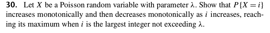
Notation:Poi$(\lambda),$ where $\lambda > 0.$
Sample space: {0,1,2,...}
PMF:
$$
P(X=x) = \left\{\begin{array}{ll}
e^{-\lambda}\cdot\frac{\lambda^x}{x!} &\text{if }$x=0,1,2,...$\\
0 &\text{otherwise.}
\end{array}\right.
$$
Terminology: Such an $X$ is said to have (or follow) Poi$(\lambda)$
distribution. We also say that $X$ is a Poi$(\lambda)$ random
variable, and write $X\sim$Poi$(\lambda).$
::
EXERCISE 11: (Easy)
If $X\sim$Poi$(3),$ then find the following probabilities.
$(1+e^{-10})/2$ [Thanks to Mayukh for correcting a typo here.]
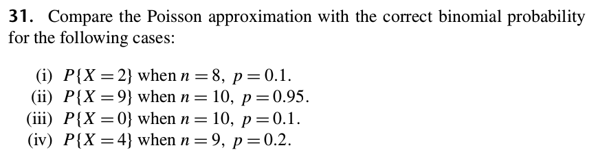
Where used: One use of Poisson distribution is in approximating
Binomial distribution.
EXAMPLE 4:
$X$ has Bin(1000,0.01) distribution. Compute $P(X=5)$
approximately by using Poisson approximation.
SOLUTION: Here $n=1000$ and $\lambda = 0.01.$ So we should take $\lambda
= 1000\times 0.01 = 10.$ By Poisson approximation, $X$ is
approximately a Poi(10) random variable. Hence
$$
P(X=5)\approx e^{-10}10^{5}/5! = 0.03783.
$$
It is instructive to compare this with the exact value, which is
$$
P(X=5) = {1000\choose 5} (0.01)^5(1-0.01)^{1000-5} = 0.03745.
$$
■
::
EXERCISE 13: (Medium)
A box has 100 items, each of which either passes a quality control test
(OK) or fails the test (BAD). If a box has more than 3 BAD items, then the
box is rejected by the quality control inspector. It is known that each
item is BAD with probability 0.01, and that the items are independent. Use
Poisson approximation to compute the probability that a box is not
rejected.
Expectation and variance: If $X$ has Poi$(\lambda)$
distribution then
$$\begin{eqnarray*}
E(X)&=&\lambda\\ Var(X)& =& \lambda.
\end{eqnarray*}$$
$$\begin{eqnarray*}
E(X) &=& \sum_{x=0}^\infty xP(X=x)\\
&=& \sum_{x=0}^\infty x\frac{e^{-\lambda}\lambda^x}{x!}\\
\end{eqnarray*}$$
The term for `$x=0$' is zero in this sum. So we can drop it to get
$$\begin{eqnarray*}
\sum_{x=0}^\infty x\frac{e^{-\lambda}\lambda^x}{x!}
&=& \sum_{x=1}^\infty x\frac{e^{-\lambda}\lambda^x}{x!}\\
&=& e^{-\lambda}\sum_{x=1}^\infty x\frac{\lambda^x}{x!}\\
&=& e^{-\lambda}\sum_{x=1}^\infty \frac{\lambda^x}{(x-1)!}\\
\end{eqnarray*}$$
Now put $y=x-1.$
$$\begin{eqnarray*}
e^{-\lambda}\sum_{x=1}^\infty \frac{\lambda^x}{(x-1)!}
&=& e^{-\lambda}\sum_{y=0}^\infty \frac{\lambda^{y+1}}{y!}\\
&=& e^{-\lambda}\lambda\sum_{y=0}^\infty \frac{\lambda^{y}}{y!}\\
&=& e^{-\lambda}\lambda e^\lambda\\
&=& \lambda.
\end{eqnarray*}$$
$$\begin{eqnarray*}
E(X(X-1))&=& \sum_{x=0}^\infty x(x-1)P(X=x)\\
&=& \sum_{x=0}^\infty x(x-1)\frac{e^{-\lambda}\lambda^x}{x!}\\
\end{eqnarray*}$$
Drop the first two terms (which are both zeroes) to obtain
$$\begin{eqnarray*}
\sum_{x=0}^\infty x(x-1)\frac{e^{-\lambda}\lambda^x}{x!}
&=& \sum_{x=2}^\infty x(x-1)\frac{e^{-\lambda}\lambda^x}{x!}\\
&=& e^{-\lambda}\sum_{x=2}^\infty x(x-1)\frac{\lambda^x}{x!}\\
&=& e^{-\lambda}\sum_{x=2}^\infty \frac{\lambda^x}{(x-2)!}\\
\end{eqnarray*}$$
Substitute $y=x-2$ to see that
$$\begin{eqnarray*}
e^{-\lambda}\sum_{x=2}^\infty \frac{\lambda^x}{(x-2)!}
&=& e^{-\lambda}\sum_{y=0}^\infty \frac{\lambda^{y+2}}{y!}\\
&=& e^{-\lambda}\lambda^2\sum_{y=0}^\infty \frac{\lambda^{y}}{y!}\\
&=& e^{-\lambda}\lambda^2 e^\lambda\\
&=& \lambda^2.\\
\end{eqnarray*}$$
$$\begin{eqnarray*}
E(X^2) &=& E(X(X-1)+E(X)\\
&=& \lambda^2 +\lambda.
\end{eqnarray*}$$
$$\begin{eqnarray*}
Var(X) &=& E(X^2) - (E(X))^2\\
&=& \lambda^2 +\lambda - \lambda^2\\
&=& \lambda.
\end{eqnarray*}$$
::
EXERCISE 14: (Easy)
Find the expected values of the following random variables.
EXERCISE 16: (Easy)
If $X_1,X_2,X_3,X_4$ are independent random variables with
distributions Poi(1),Poi(2),Poi(4) and Poi(5),
respectively.
Find the distribution of $(X_1+\cdots+X_4).$
Proof:
Since $p = \frac \lambda n,$ hence
$$
\binom{n}{k} p^k (1-p)^{n-k} = \frac{n! }{k!(n-k)! }\times
\frac{\lambda^k}{n^k}\times \left(1-\frac \lambda n \right)^{n-k}.
$$
Separate out all factors free of $n$ to rewrite this as
$$
\frac{ \lambda^k}{k!} \times \frac{ n! }{(n-k)! n^k }\left(1-\frac \lambda n \right)^{n-k}.
$$
Now
$$
\left(1-\frac \lambda n \right)^{-k}\rightarrow 1,
$$
since $k$ is fixed. Also
$$
\left(1-\frac \lambda n \right)^n \rightarrow e^{-\lambda}.
$$
Finally, since $k$ is fixed, we have
$$
\frac{ n(n-1)\cdots(n-k+1) }{ n^k }\rightarrow 1,
$$
completing the proof.
[QED]
This theorem is often interpreted as: number of rare events follows Poisson distribution. This is
more of a myth than anything real. But since it is very popular belief, let me explain how this
interpretation arises:
Consider accidents occuring at a crossing. Everytime two cars come close, there is a chance of an
accident. But most of the time an accident does not occur. So we may think of "two cars coming close" as a "coin toss"
and an "accident" as "head". Since accidents are rare, we shall consider $P(H)$ to be very small. Also at a busy crossing
two cars often come close, i.e., the coin is being tossed a large number of times. With this interpretation the nuber of
accidents should follow $Binom(n,\theta)$ distribution with large $n$ and small $\theta.$ Hence $Poisson(\lambda)$
with $\lambda=n \theta$ should be a good approximation.
This interpretation is clearly an over-simplification of the situation. However, this myth is fuelled by a well-known (and
useless) data set regarding number of deaths of Prussian soldiers by kicks of their own
horses. Here is the data set. This form os death is pretty rare (thankfully!). If we make
a bar plot of the relative frequencies, we get a very good match with a Poisson distribution.
Let us find the probability that the preassigned player
has all the 4 aces in one dealing.
Step 1: Give the 4 aces to that player: 1 way
Step 2: Give the 9 more cards to that player: $\binom{52-4}{9}$ ways
Step 3: Deal the remaining 39 cards among the other 3 playes: $\frac{39!}{13!13!13!}$ ways.
Total number of ways of dealing is $\frac{52!}{13!13!13!13!}$. So the probability is $\frac{13\times\cdots\times10}{52\times\cdots\times49} = p$,
say.
Then the probability of this happening at lest once in $n$ independent dealings is $1-(1-p)^n$. We are looking
for the smallest $n$ such that $1-(1-p)^n\geq \frac 12$.
Let a random page have $X$ misprints. Then we assume $X\sim Poi(\lambda)$ for some $\lambda$. Now $E(X) = \lambda$.
We estimate $\lambda$ as $\frac{500}{500} = 1$. So the problem is to find $P(X\geq 3)$ where $X\sim Poi(1)$.
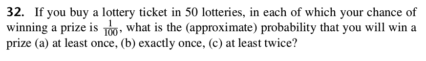
If $X$ is the number of colour-blind persons in an SRSWR of size $n$, then $X\sim Binom(n,0.01)$.
We want $n$ such that $P(X\geq 1) \geq 0.95$, i.e., $1-P(X=0) \geq 0.95$.
Let $X$ be the number of misprints in a random page. We assume $X$ has a Poisson
distribution (Texbookish weak rationale: The
page has many words, each word has a misprint or not with some probability. Assuming independence, $X$ should be binomially
distributed. Since the number of words is large, and the chance of misprints per word is small, hence we can use Poisson
approximation.)
So $X\sim Poi(\lambda)$ since $E(X) = \lambda$.
So probability that there are at least $k$ misprints in a random page is $P(X\geq
k)=1-P(X<k) = 1- e^{-\lambda}\sum_0^{k-1} \frac{\lambda^i}{i!} = p$, say.
Let $Y$ be the number of pages with at least $k$ misprints among those $n$ pages.
Assuming the numbers
of misprints in different
pages are independent, $Y\sim Binom(n,p)$.
The required probability is $P(Y\geq 1) = 1-P(Y=0) = 1-(1-p)^n$.
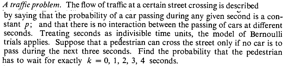
Think of the problem like this: The god of traffic is tossing a coin with $P(H)=p$
repeatedly (and independently), resulting in a sequence of H's and T's. The pedestrian can view the sequence at least 3
steps into the future. Thus, initially he knows at least first three outcomes, then in the next second he knows at least
the first four outcomes, and so on. He would cross if an only if the next 3 outcomes are all tails.
With this formulation waiting for 0 second is having TTT. Waiting for
exactly 1 second is having HTTT, and so on. Waiting for 2 seconds correspond to {HHTTT, THTTT} but not to HTTTT.
[Thanks to Souradip for pointing out a mistake here.]
Let $X,Y$ be the their numbers of heads (I mean
of their tosses, not their own!) Then $X,Y$ are IID $Binom\left(n,\frac 12\right)$. Find
$P(X=Y) = \sum_0^n P(X=k)^2=\cdots.$.
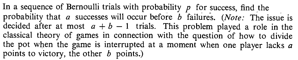
Let $X$ be the number of trials needed to get the first $a$ successes. Then $X\sim
NegBin(p,a)$. We are looking for $P(X<a+b)$.
This may also be computed directly by considering all possible success-failure sequences of length
$a+b-1$ and locating the sequences favourable to our event (i.e., all sequences with at
least $a$ successes).
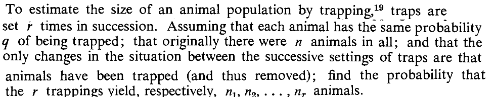
Let $X_i = $ number of animals trapped in the $i$-th trapping.
Then $X_1\sim Binom(n,q)$, $X_2|X_1\sim Binom(n-X_1,q)$, $X_3|X_1,X_2\sim Binom(n-X_1-X_2,q)$, etc.
We have to find $P(\forall i~~X_i = n_i) = P(X_1=n1)P(X_2=n_2|X_1=n_1)P(X_3=n_3|X_1=n_1,\,X_2=n_2)\cdots$.
::
EXERCISE 29: (Medium)An insect lays $X$ eggs where $X\sim Poi(\lambda)$. Each of the eggs may hatch or perish independently
of the others. The chance of a random egg hatching is $p$. Let $Y$ be the total number of eggs
that hatch. Show that
$Y\sim Poi(\lambda p)$.
The first inequality follows from $n(n-1)\cdots(n-k+1) \geq n^k$.
The second follows from $n(n-1)\cdots (n-k+1) \leq (n-k)^k$.
::
EXERCISE 31: (Medium)Use the above inequality to show that
$$
\frac{e^{-\lambda}\lambda^k}{k!} e^{k \lambda/n}
>
\binom{n}{k}p^k(1-p)^{n-k}
>
\frac{e^{-\lambda}\lambda^k}{k!} e^{-k^2/(n-k)-\lambda^2/(n-\lambda)}.
$$
For the first inequality use the fact that $\log(1+x) < x$ for $|x| < 1$.
For the second use the fact that $\log(1+x) > x-\frac{x^2}{2}$ for $|x| < 1$. You may also proceed using just $e^x > 1+ x$
for $x >0$.
::
EXERCISE 32: (Hard)(Banach's matchbox problem)
A certain mathematician has two matchboxes (containing $n$
matches each), one in his left pocket, the other in the
right. When he needs to light a cigar (smoking which, BTW, is
injurious to health) he chooses one of the two pockets at random,
and takes a match from the box in that pocket. (Choices of
pockets are assumed independent.) One day for the first time he
discovers that his chosen box is empty. What is the probability
distribution of the number ($X$) of matches remaining in
the other box? [Hint: To get yourself started first
find $P(X=n).$ This means he has been using the same
box $n$ times without ever using the other box.]
Let's work out $P(X=3)$ when $n=5$. This means he has already used up 7 matches (5 matches from the
current pocket and 5-3=2 matches from the other). So this must be his 8th search. Each of these
8th searches was either in his left (L) or right (R) pocket. So there are $2^8$ ways in all.
Now let us count the outcomes leading to our event. Exactly half of these end with L, the other
half ending with R. Let's count the ones ending with L. There must be exactly 5 L's among the
first 7 entries. So the total numbr is $\binom75$.
Hence $P(X=3) = \frac{2\binom75}{2^8}$.


 Use Poisson distribution.