For many random variables we see a striking example of
statistical regularity. As an example, consider this gambling game:
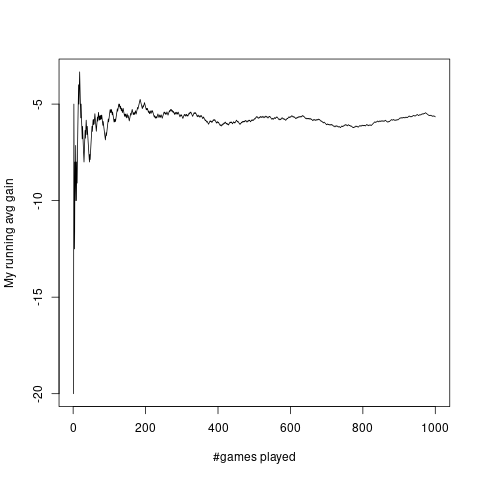
A fair die is rolled. If it shows an odd number then I pay you Rs 20, else you pay me Rs 10.
A typical plot of my running average gain per game against number of games is as follows:
It is produced by the following code.
w = sample(6,1000,rep=T)
profit =c(-20,10,-20,10,-20,10)
X = profit[w]
avgX = cumsum(X)/(1:1000)
#png('image/explotnow.png')
plot(avgX,ty='l',xlab="#games played",ylab="My running avg gain")
#dev.off()
In fact, it is this phenomenon that first let man to study
probability. If you run a gambling game a large number of time
the running average profit per game becomes more and more stable. Gamblers wanted
to guess this stable value beforehand. They argued as follows:
If I play this game a large number of times (say $n$ times),
then
approximately $\frac n2$ times I should get $10$
and the remaining $\frac n2$ times I should get $-20.$ So
approximately my total gain would be
$$
\frac n2\times 10 + \frac n2\times (-20).
$$
So the average should be approximately this divided by $n,$
i.e.,
$$
\frac 12\times 10 + \frac 12\times (-20) = -5.
$$
Indeed, this simple argument turns out to be remarkably
accurate. Gamblers could not understand why it becomes so
accurate as $n$ becomes large. But nevertheless they used this formula to
find out what they could expect the random variable to do in the
long run.
A random variable is called simple if takes only finitely many values.
::
EXERCISE 1: (Easy)A random variable $X$ takes the values $-2, -1, 0, 1 $ and $2$ with
probabilities $p,q,1-2p-2q, p$ and $q,$ respectively. Find $E(X).$
::
EXERCISE 2: (Easy)A random variable takes the values $1,2,...,10$ with probabilities
$p_1,p_2,...,p_{10},$ respectively, where $\sum_i p_i = 1.$ Prove that $1\leq
E(X)\leq 10.$ Also find $p_i$'s if $E(X) = 10.$
For any random variable $X$ we define $X_+ =
\max\{X,0\}$ and $X_- = -\min\{X,0\}.$ Notice that
both $X_+$ and $X_-$ are nonnegative.
EXERCISE 3: (Easy)Which of the following must be true?
$X = X_++X_-.$
$X = X_+-X_-.$
$X = X_--X_+.$
None of the above.
Notice that we leave the case $E(X_+), E(X_-)=\infty $
unmentioned in the definition. This means $E(X)$ is
undefined in this case.
EXAMPLE 1: A random variable takes the values $\pm 2^n$ for $n\in{\mathbb N}$ with probabilities
$P(X=2^n) = P(X=-2^n) = 2^{-n-1}$ for $n\in{\mathbb N}$. What is $E(X)$?
SOLUTION:
Here $X_+$ takes the values 0, 2, $2^2, 2^3,...$ with probabilities $2^{-1}, 2^{-2}, 2^{-3},...$.
So $E(X_+) = 0 + \frac 12+\frac 12+\frac 12+\cdots = \infty$.
Similarly, $E(X_-) = \infty$.
Hence $E(X)$ is undefined.
■
It is possible to define expectation of random variables that are more general (taking uncountably many values). We shall
give most general definition in the next semester. The following properties actually hold for the genral definition.
Unless noted otherwise, we
shall only prove them for the case of simple random variables. These proofs are actually the first steps in the general proofs
that will come next semester.
Many students somehow get the idea that if a (discrete) random variable $X$ takes
the values $x_1,x_2,..$. with probabilities $p_1,p_2,...$ where $\sum p_i = 1$,
then $E(X) = \sum_i x_i p_i$. But this is wrong! It is wrong even if the sum converges!
This formula is true in the following special cases:
If $X$ is simple, i.e., takes only finitely many values.
If $X$ takes only nonnegative (or only nonpositive) values (and here the formula holds even if the sum
diverges).
If $\sum_i |x_i| p_i < \infty$.
Here is another point that students sometimes get wrong. When we say $E(X)$ is undefined we mean $E(X)$
is meaningless in that context, and not that $E(X)$ can be anything there.
The condition "$X$ always lies in $[a,b]$" may be
written as $P(X\in[a,b])=1.$
Proof:
Here $X\leq Y$ means $\forall \omega\in\Omega~~X(\omega)\leq Y(\omega).$
As already mentioned, we shall restrict the proof to only the case where $X$ and $Y$ are both simple.
Let $X$ take values $x_1,...,x_m,$ and $Y$ take values $y_1,...,y_n.$
Let $p_{ij} = P(X=x_i, Y=y_j).$
Clearly, if $p_{ij}>0,$ then we must have $x_i\leq y_j.$
Now
$$\begin{eqnarray*}E(X) & = & \sum_i x_i P(X=x_i) = \sum_i (x_i \sum_j p_{ij}) =\sum_i\sum_j (x_i p_{ij})\\
& \leq & \sum_i\sum_j (y_j p_{ij}) ~~[\because p_{ij}>0\Rightarrow x_i\leq y_j]\\
& = & \sum_j\sum_i (y_j p_{ij})[\because \mbox{addition is associative and commutative}]\\
& = & \sum_j (y_j \sum_i p_{ij}) = \sum_j y_j P(Y=y_j) = E(Y).
\end{eqnarray*}$$
[QED]
EXERCISE 4: (Easy)Prove this for simple $X$.
However, if $a\in{\mathbb R}$ is replaced by $\infty,$ then the
result fails, i.e.,
It is possible to have a random
variable $X$ that is always finite (any real-valued random
variable will do, since $\infty\not\in{\mathbb R}$) such
that $E(X)=\infty.$ Of course, we cannot get a counterexample using simple random variables.
However, such counterexamples exist for random variables taking countably many values, as shown below.
EXAMPLE 2:
It is a standard fact that $\sum\frac{1}{n^2}<\infty.$ Let the
sum be $c.$ (The exact value of $c$
which is $\frac{\pi^2}{6},$ is of no importance here).
Then consider a random variable $X$ that takes values
in ${\mathbb N}$ and $P(X=n)=\frac{1}{cn^2}.$
Then $E(X) = \frac 1c\sum\frac 1n=\infty.$
■
By the way, if $X$ can take values $x_1,x_2,...$, there
is no guaranty that $E(X)$ will equal any of
the $x_i$'s. For example, if $X$ is the outcome of
a fair die, then $E(X)=3.5,$ which is not a possible
outcome.
EXERCISE 5: (Easy)
If $E(X) = \mu\in{\mathbb R},$ then what is $E(X-\mu)?$
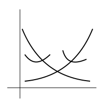
Next we shall need a new concept, that of a convex
function. Graphically, $f(x)$ is a convex function if its
graph is like a bowl opening upwards (possibly slanted). Some
examples are shown below.
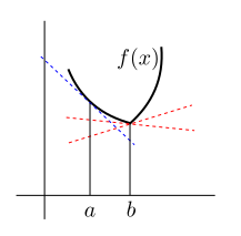
Mathematically we may define a convex function as follows.
While this definition is graphically quite intuitive, you
may have seen other definitions of convexity
elsewhere. Read here to learn more
about equivalences between different definitions of convexity.
In the following diagram the blue line is $\ell_a.$ Both the
red lines are candidates for $\ell_b.$
Proof:
Let $\mu = E(X).$ Consider $\ell_\mu(x)$ as mentioned
in the definition of convexity.
Since the graph of $\ell_\mu(x)$ is a straight line passing
through $(\mu,f(\mu)),$ hence it must be of the form
$$\ell_\mu(x) = f(\mu)+m(x-\mu),~~x\in{\mathbb R}.$$
So
$$
E(f(X)) \geq E(\ell_\mu(X)) = E(f(\mu))+mE(X-\mu) = f(\mu)+0 = f(E(X)),
$$
as required.
[QED]
::
EXERCISE 6: (Medium)Which is larger $(E(X))^2$ or $E(X^2)?$ Assume
that both exist finitely.
EXAMPLE 3:
Suppose I have a random variable that takes values $-1,0$ and $1$
with probabilities $0.1, 0.5$ and $0.4,$ respectively.
What is $E(X^2)?$
SOLUTION:
Here $X^2$ is a new random variable. Call it $Y,$ say. Then $Y$
takes values $0$ and $1$ with probabilities $0.5$
each.
So $E(Y) = \frac 12.$
■
Here is another technique to arrive at the same result.
$$
E(X^2) = 0.1\times (-1)^2 + 0.5\times 0^2 + 0.4\times 1^2 = 0.5.
$$
This technique is often easier because here we do not need to
find the distribution of $Y=X^2$ first. Both these
techniques will always give the same answer.
Proof:
If $X$ takes only finitely many values, then the result
follows from distributivity of multiplication over addition.
If $X $ takes countably infinitely many values, and $h(X)$ is non-negative, then define
$$
U_n =\left\{\begin{array}{ll}h(X)&\text{if }X=x_1,...,x_n\\ 0&\text{otherwise.}\end{array}\right.
$$
and proceed as for the proof of $E(X)=\sum p_i x_i.$
[QED]
Often we have to find $E(X)$ where $X$ is the count of something, e.g., number of heads in 100 tosses of coin,
or number of times something interesting happens. If you want to find $E(X)$ directly from the definition, then you
need to find the distribution of $X$ first, which is often difficult. In such situatons the
indicator trick may provide a short cut.
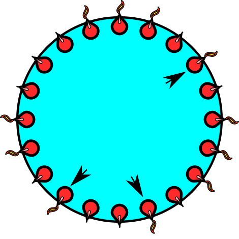
EXAMPLE 4: We have a ring of 20 lamps. A wind blows and a random subset of lamps go out. Find
the expected number of singleton lights (i.e., lighted lamps with both neighbours off).
The singletons are shown with arrowheads
SOLUTION:
Let $X$ be the number of singletons. Finding the distribution of $X$ is not very difficult, but still we shall
demonstrate the use of the indicator trick.
We shall use the arrowheads as our random variables. Let the lamps be numbered from 1 to 20. Define $L_i=1$
if $i$-th lamp is on and is a singleton, and $0$ else. In other words, $L_i=1$ means we have put an
arrow head at position
$i.$
Each $L_i$ is called an indicator variable.
Clearly $X = L_1+\cdots+L_{20}.$
So $E(X) = E(L_1)+\cdots+E(L_{20}) = 20 E(L_1),$ since by symmetry all the $L_i$'s have the same distribution.
To find $E(L_1)$ we need to find just $P(L_1=1)$, which involves only lamp 1 and its two neighbours. It should
be clear that $P(L_1) = \frac{1}{8}.$
Hence $E(X) = \frac{20}{8} = \frac 52.$
■
We know from the definition of expectation that it may come in four varieties: it may be finite, or $\infty$ or $-\infty$
or undefined.
The finite case is the most useful, and it
sometimes helps to know some sufficient conditions for this.
Proof:
Goes without saying!
[QED]
Non-negative random variables have the advantage that their expectation is always defined (though may be $\infty$). Now,
from any random variable $X$ we can easily manufacture a non-negative random variable, viz, $|X|.$ It is
good to be able to relate $E(X)$ with $E(|X|).$
Proof:
We define $X_+, X_-$ as usual.
Then $X = X_+-X_-$ and $|X| = X_++X_-$.
Then finiteness of $E(|X|)$ is equivalent to finiteness of both $E(X_+), E(X_-).$
Again, finiteness of $E(X)$ is equivalent to finiteness of both $E(X_+), E(X_-).$
Hence the result.
[QED]
::
EXERCISE 7: (Medium)If $E(|X|)=\infty,$ then what can you say about $E(X)?$
Proof:
Since $E(Y)$ is finite, hence $E(|Y|)$ is finite. So $E(|X|)\leq E(|Y|)$
is also finite. Hence $E(X)$ is finite.
[QED]
Proof:Step 1: First we shall prove it for nonnegative $X,Y$. Since $E(X)$ and $E(Y)$ are both finite,
so must be $E(X+Y)$.
Now, thanks to nonnegativity of $X,Y$ we must have $\max\{X,Y\}\leq X+Y$.
So, by the last theorem, $E(\max\{X,Y\})$ must be finite.
Step 2: Apply step 1 to $|X|$ and $|Y|$ and use the fact that
for any $a,b\in{\mathbb R}$ we have $|\max\{a,b\}|\leq \max\{|a|,|b|\}$.
[QED]
It is possible to combine the two steps into a single line proof. But stepwise thinking starting with the nonnegative case
is a good habit.
Proof:
Use the fact that $|X^m| \leq \max\{1,|X^n|\}.$ Now use the
last theorem.
[QED]
The following theorem often proves very useful.
Proof:
Let $Y =\left\{\begin{array}{ll}\epsilon&\text{if }X\geq \epsilon\\ 0&\text{otherwise.}\end{array}\right.. $
Then clearly, $X\geq Y$. So $E(X)\geq E(Y) = \epsilon P(X\geq \epsilon)$.
[QED]
EXERCISE 9: (Medium)Show that if $X$ is a random variable taking only non-negative
integer values, then
$$E(X) = \sum_{k=1}^\infty P(X\geq k).$$
This formula often proves useful for finding expected counts.
Let $p_n = P(X=n)$ for $n=0,1,2,3,...$
Then
$$\begin{eqnarray*}
P(X\geq 1) & = & p_1 + p_2 + p_3+\cdots\\
P(X\geq 2) & = & \phantom{p_1 +} p_2 + p_3+\cdots\\
P(X\geq 3) & = & \phantom{p_1 + p_2 +} p_3+\cdots\\
\cdots
\end{eqnarray*}$$
Now add columnwise. Non-negative series do not change value when
you rearrange the terms.
::
EXERCISE 10: (Medium)For a group of $n$ people find the expected number of days of the year which are
birthdays of exactly $k$ people. (Assume 365 days and that all arrangements are equally
probable.) Also find the expected number of multiple birthdays. How large should $n$ be to
make this expectation exceed 1?
Let $X_i = \left\{\begin{array}{ll}1&\text{if }\mbox{exactly $k$ people have birthdays on day} i\\ 0&\text{otherwise.}\end{array}\right..$
Then $X = \sum_1^{365} X_i.$
So $E(X) = \sum_1^{365} E(X_i).$
Expected number of days of the year which are birthdays of exactly $k$ people is $\binom{n}{k}\frac{364^{n-k}}{365^{n-1}}.$
Expected number of multiple birthdays is $365\left\{1-\left(\frac{364}{365}\right)^n - \frac{n\times 364^{n-1}}{365^n}\right\}.$
::
EXERCISE 11: (Medium)A man with $n$ keys wants to open a door (where exactly one key works). He tries the
keys independently at random. Find the expected number of trials needed to open the door if
keys are tried (a) with replacement (b) without replacement.
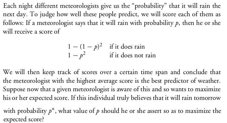
Here $p$ is what he says, and $p^*$ is what he believes. The meteorologist is not an honest one, and may
say something different from what he believes. His only aim is to maximise the expected score.
The expected score is
$$p^*(1-(1-p)^2) + (1-p^*)(1-p^2).$$
This is to be maximised wrt $p$ (with $p^*$ fixed).
Differentiate (or think of the graph) to see that the maximising value of $p$ is $p^*.$
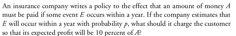
Company pays the amount $A$ with probability $p.$ It pays $0$ with probability $1-p.$
So its expected payoff is $pA.$
Suppose that it charges $B.$ Then expected profit is $B-pA.$ To keep it 10% of $A$ we need $B = (p+0.1)A.$
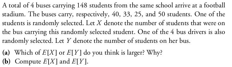
(a) $E(X)$ would be larger, because when a student is selected at random, he is more likely to come from the larger
buses. So $E(X)$ is a weighted average of the bus sizes where the larger buses get more weight.
But $E(Y)$ is the simple average of the bus sizes.
(b) $E(X) = \frac{40^2+33^2+25^2+50^2}{40+33+25+50}.$
$E(Y) = \frac{40+33+25+50}{4}.$
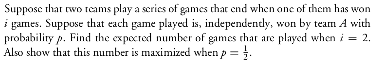
By the pigeon hole principle, the winner will be decided by at least 2 and at most 3 games.
So the sample space is $\{AA, BB, ABA, BAA, BAB, ABB\}.$ The probabilities are, respectively,
$p^2, q^2, p^2q, p^2q, pq^2, pq^2,$ where $q=1-p.$
If $X$ is the random variable denoting the number of
games played, then it takes the values, respectively, $2,2,3,3,3,3.$
So $E(X) = 2(p^2 + q^2) + 3(2p^2q + 2pq^2) = 2(1+pq).$
This is maximised when $pq = p(1-p)$ is maximised, which is when $p=\frac 12.$
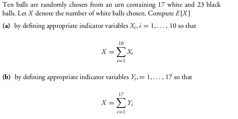
(a) Let $X_i = \left\{\begin{array}{ll}1 &\text{if }i\mbox{-th draw is white}\\ 0&\text{otherwise.}\end{array}\right.$ for $i=1,...,10.$
Then $E(X_i) = P(i$-th draw is white$)=\frac{17}{40}.$
So $E(X) = 10\times \frac{17}{40} = \frac{17}{4}.$
(b) Let $Y_i = \left\{\begin{array}{ll}1&\text{if }i\mbox{-th white ball is selected}\\ 0&\text{otherwise.}\end{array}\right.$ for $i=1,...,17.$
Then $E(Y_i) = P(i$-th white ball is delected$)=\frac 14.$
So $E(X) = 17\times \frac 14 = \frac{17}{4}.$
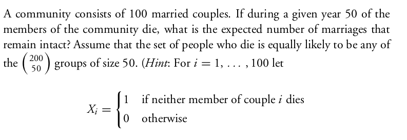
Let $X_i$ be as given in the hint.
Let $X = $ number of intact marriages.
Then $X = \sum_1^{100} X_i$
Now $E(X_i) = \binom{198}{50}/\binom{200}{50}=\frac{150\times149}{200\times199}.$
So $E(X) = \frac{150\times149}{2\times199}.$
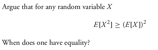
Here we assume that $E(X)$ exists finitely. The inequality holds even if
$E(X^2)$ is not finite (with the interpretation that $\forall a\in{\mathbb R}~~\infty \geq a$.)
You may either use Jensen's inequality with the convex function $f(x)=x^2$ or the fact that $V(X)\geq 0.$
Equality if and only if $V(X)= 0$, i.e., if $X$ is a degenerate random variable.
::
EXERCISE 21: (Hard)
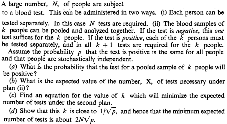
You may use some approximations in parts (c) and (d) of this problem. For instamce there are
$\frac nk$ groups of $k$ patients each, even if $\frac nk$ is not an integer. You
may also differentiate w.r.t. $k.$
(a) $1-(1-p)^k.$
(b) For a group of size $k$ the random variable $X$ takes the value
$k+1$ with probability $1-(1-p)^k$ and the value $1$ with probability $(1-p)^k.$
So $E(X) = (k+1)(1-(1-p)^k)+(1-p)^k = k+1-k(1-p)^k.$
If there are $N$ people in all, where $N = qk+r$ with $r\in\{0,...,k-1\}$,
then this applies to each of the $q$ groups and also the reaminder group of size $r.$
So the required expectation is
$$q(k+1-k(1-p)^k)+r+1-r(1-p)^r.$$
If $k$ divides $N$, then this is
$$\frac Nk(k+1-k(1-p)^k) = N+\frac Nk-N(1-p)^k = N\left(1+\frac 1k-(1-p)^k\right).$$
(c) Enough to minimise $1+\frac 1k-(1-p)^k$ wrt $k$ for given $p.$
Treating $k $ as a continuous variable, the derivative is
$$-\frac{1}{k^2}-(1-p)^k\log(1-p).$$
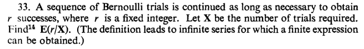
Here $P(X=k) = \binom{k-1}{r-1}p^rq^{k-r}$ for $k=r,r+1,...$ where $q = 1-p.$
So
$$E\left(\frac rX\right) = \sum_{k=r}^\infty \binom{k-1}{r-1}p^rq^{k-r}\frac rk.$$
This may be handled by repeated term by term integration and differentiation of the power series
$$1+q+q^2+\cdots = \frac{1}{1-q}$$
for $|q|<1.$
For example, if $r=1$, then the sum is
$$p\sum_{k=1}^\infty \frac{q^{k-1}}{k} = \frac pq\sum_1^\infty \frac{q^k}{k} = \frac pq\sum_1^\infty \int_0^q t^{k-1}\, dt =
\frac pq\int_0^q \sum_1^\infty t^{k-1}\, dt =\frac pq\int_0^q \frac{dt}{1-t} = \cdots. $$
Let $X = $ the number of trials needed to get the first 6.
Then $P(X=k) = \left(\frac 56\right)^{k-1}\frac 16$ for $k=1,2,3,....$
So $E(X) = \sum_{k=1}^\infty k \left(\frac 56\right)^{k-1}\frac 16.$
Now, we know that $\frac{1}{1-x} = 1+x+x^2+x^3+\cdots$
if $|x|<1.$ This may be differentiated term by term (needs a justification that you should learn in your real analysis
class) to give
$$\frac{1}{(1-x)^2} = 1+2x + 3x^2+\cdots.$$
Put $x=\frac 56$ to find the required expectation.
Assuming the dice to be fair, the answer does not depend on the number
the gambler bets on.
Let $X$ be the loss for unit stake on 1.
Then
$$X = \left\{\begin{array}{ll}
1&\text{if }\mbox{no die shows 1}\\
-1&\text{if }\mbox{exactly 1 die shows 1}\\
-2&\text{if }\mbox{exactly 2 dice show 1}\\
-3&\text{if }\mbox{all 3 dice show 1}\\
\end{array}\right..$$
So $P(X=1) = \left(\frac 56\right)^3$, $P(X=-1) = 3\left(\frac 16\right)\left(\frac 56\right)^2$,
$P(X=-2) =
3\left(\frac 16\right)^2\left(\frac 56\right)$ and $P(X=-3) = \left(\frac 16\right)^3.$
Hence
$$E(X) = \left(\frac 16\right)^3(5^3-3\times 5^2-6\times5-3).$$
Let $T_1 = 1.$
Let $T_i = $ waiting time for the $i$-th new coupon after the $(i-1)$-th coupon has been encountered, for
$i=2,3,4,5.$
Consider the following example to understand the definition of $T_i$'s. Suppose that the coupons arive in the order:
3 3 4 3 5 4 3 4 2 3 4 5 1.
The first occurences of each type of coupon have been shown in red. They are at positions
$$S_1 = 1, S_2 = 3, S_3 = 5, S_4=9\mbox{ and } S_5=13.$$
We are defining $T_i = S_i-S_{i-1}$ for $i=1,...,5$ where $S_0=0.$
Then the $T_i$'s are independent random variables.
$T_1$ is degenerate at 1, and for $i=2,...,5$ we have
$$P(T_i = k) = q_i^{k-1}p_i$$ for $k\in{\mathbb N}$ where $q_i = \frac{i-1}{5}$ and $p_i = 1-q_i.$
We can easily find $E(T_i)$'s.
The answer to the problem is $E(T_1+\cdots+T_5) = 1+E(T_2)+\cdots+E(T_5).$
[Thanks to Nipam for correcting a mistake here.]
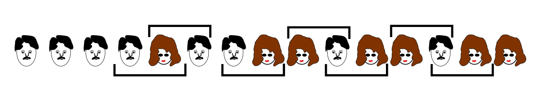
The same person may be part of two marriageable couples.
The guys are all distinct, and so are the girls (though it is not clear from my wonderful artwork!).
The diagram shows 8 runs, i.e., stretches of same gender. A single girl or a single guy consitute the shortest possible
run. Notice that the number of marriageable couples is one less than the number of runs.
Thus, the number of arrangements with $k$ marriageable couples is
the same as the number of arrangements with $k+1$ runs.
Here $k$ can take any value between $1$ and 14.
As an example let us find $P(k=3).$
The total number of arrangements is of course $15!.$
We need $3+1=4$ runs: either male-female-male-female or female-male-female-male.
Step 1: Arrange the guys: 8! ways
Step 2: Arrange the girls: 7! ways
Step 3: Insert a separator to split the guys into two runs: 7 ways
Step 4: Insert a separator to split the girls into two runs: 6 ways
Step 5: Mix them: 2 ways (M-F-M-F or F-M-F-M)
So
$$P(k=3) = \frac{8!\times7!\times7\times6\times2}{15!}.$$
Find these for all possible values $k$, and then compute expectation.
Or...use the indicator trick!!!
Let there be $n$ workers. Let $X$ be the number of working days.
Let $X_i=\left\{\begin{array}{ll}1&\text{if }i\mbox{-th day is a working day}\\ 0&\text{otherwise.}\end{array}\right..$
Then $X = \sum_1^{365} X_i.$
Now $E(X_i) = P(i$-th day is a working day$)= \left(\frac{364}{365}\right)^n.$
So $E(X) = 365\times \left(\frac{364}{365}\right)^n.$
Hence expected number of man-days is
$365n\times \left(\frac{364}{365}\right)^n=f(n)$, say.
We want to maximise this wrt $n.$
Now
$$\frac{f(n+1)}{f(n)} = \frac{n+1}{n}\times \frac{364}{365}.$$
This is $>/=/< 1$ according as $364 >/+/< n.$
So the function is maximised at $n=364$ and $365.$
Let $X=$ number of cards required to be turned.
Then $P(X=k)=\frac{4\times {}^{48}P_{k-1}(52-k)!}{52!}.$
So you can now find $E(X) = \sum_{k=1}^{49} k P(X=k)$.
But here is a smarter solution (taken from Mosteller's book and also given by a student via Whatsapp):
 Many students somehow get the idea that if a (discrete) random variable $X$ takes
the values $x_1,x_2,..$. with probabilities $p_1,p_2,...$ where $\sum p_i = 1$,
then $E(X) = \sum_i x_i p_i$. But this is wrong! It is wrong even if the sum converges!
This formula is true in the following special cases:
Many students somehow get the idea that if a (discrete) random variable $X$ takes
the values $x_1,x_2,..$. with probabilities $p_1,p_2,...$ where $\sum p_i = 1$,
then $E(X) = \sum_i x_i p_i$. But this is wrong! It is wrong even if the sum converges!
This formula is true in the following special cases: