A random variable is, well, random. So it may very well differ from
its expectation. By how much? A lot or a little? We can use
expectation to find that out.
Define
$$
Y = \left\{\begin{array}{ll}
\epsilon^2 &\text{if }|X-E(X)|\geq \epsilon\\
0 &\text{otherwise.}
\end{array}\right.
$$
Then $(X-E(X))^2\geq Y.$
So
$$\begin{eqnarray*}
V(X)
& = & E(X-E(X))^2\\
& \geq & E(Y)\\
& = & \epsilon^2 P(|X_i-E(X)| \geq\epsilon) + 0\times P(|X_i-E(X)| <\epsilon).
\end{eqnarray*}$$
Hence the result.
[QED]
A point about the inequalities in the above theorem. There are two inequalities, one inside the probability, and one outside.
Both are mixed inequalities. Obviously, you may make the first inequality strict (thereby
weakening the result). However, you may not replace the other inequality with a strict one, because otherwise you will
get $0 < 0$ for a degenerate $X$.
Proof:
We shall not do the proof here. But here is the main idea:
$$
e^{tX} = 1 + \frac{tX}{1!} + \frac{t^2X^2}{2!} + \frac{t^3X^3}{3!} + \cdots.
$$
From this we want to write
$$
E(e^{tX}) = 1 + \frac{tE(X)}{1!} + \frac{t^2E(X^2)}{2!} + \frac{t^3E(X^3)}{3!} + \cdots.
$$
This is not a precise statement, because we do not know if all
raw moments of $X$ exist finitely. Also, even if they do, is
it valid to "distribute" expectation over an infinite sum?
Answers to these questions require deeper real analysis results
than we know at this point.
However, assuming that this is valid, we may try to differentiate
both sides to get
$$
\frac{d}{dt} E(e^{tX}) = E(X) + \frac{2tE(X^2)}{2!} + \frac{3t^2E(X^3)}{3!} + \cdots.
$$
Again this step needs justification. Can we "distribute"
differentiation over an infinite sum?
Assuming that we can, puting $t=0$ indeed gives us $E(X).$
SImilarly, differentiating once again, and putting $t=0$
gives us $E(X^2),$ and so on.
[QED]
We shall not spend much time with MGFs, because there is a better
alternative called the characteristic function (CF).
Don't be nervous to see expectation of a complex random
variable. It is simply
$$
E(\cos tX) + i E(\sin tX).
$$
CFs are better than MGFs because of two reasons, that we give as
theorems below.
Proof:
This is obvious, since $\sin tX$ and $\cos tX$ are both
bounded random variables, and hence have finite expectations.
[QED]
Proof:
Not in this course.
[QED]
Indeed, this property has earned characteristic functions their name.
MGFs do not have this proprty. It is possible to get (rather
ugly) counter-examples of random variables $X$ and $Y$
that both have the same MGF (in particluar both have the same
domain $D\subseteq{\mathbb R}$), but still $X$ and $Y$ have
different distributions. However, if the domain includes a
neighbourhood of $0,$ then $X,Y$ must have the same
distribution. This is stated in the following theorem.
Proof:
Too difficult for this course.
[QED]
We shall not spend time proving any result on MGF here. You will
learn the proofs for CFs in the third semester.
EXERCISE 1: (Easy)A box has 6 red balls an 4 black balls. An SRSWR of
size $n$ is selected. If $X$ is the number of red
balls selected, then find PMF of $X$ and $E(X).$ Also solve the
problem in the case of SRSWOR.
For SRSWR: $P(X=x) = \binom{n}{x} \left(\frac{6}{10}\right)^x\left(\frac{4}{10}\right)^{n-x}$ for $x=0,1,...,n.$
For SRSWOR:
$P(X=x) = \frac{\binom{6}{x} \binom{4}{n-x}}{\binom{10}{n}}$
for $x=0,1,...,n.$
By the way, this does not mean that $X$ can indeed take all the values from 0 to $n.$ For some of these values
the probability is zero.
::
EXERCISE 2: (Easy)Let $N$ be a positive integer. Let
$$
f(x) = \left\{\begin{array}{ll}c 2^x &\text{if }x=1,2,...,N\\0&\text{otherwise.}\end{array}\right.
$$
be a PMF. Find $c.$ Find $E(X)$ and $V(X)$ if $X$ has this PMF.
For $f(x)$ to be a PMF we need
$$f(1)+\cdots+f(N)=1.$$
Hence
$$c = \frac{1}{2^{N+1}-2}.$$
So
$$E(X) = \sum_1^N x f(x) = c\sum_1^N x 2^x = ...$$
Similarly, you can find $V(X).$
::
EXERCISE 3: (Medium)An SRSWR of size 2 is drawn from $\{1,2,...,12\}.$
Let $X$ be the maximum of the two numbers
selected. Find $E(X).$
Here $X$ can take only the values $1,2,...,12.$
For $k\in\{1,2,...,12\}$ we have
$$P(X\leq k) = P(X_1, X_2 \leq k) = \left(\frac{k}{12}\right)^2.$$
So $P(X=k) = \frac{k^2-(k-1)^2}{144} = \frac{2k-1}{144}.$
Hence $E(X) = \sum_1^{12} \frac{2k^2-k}{144}=....$
::
EXERCISE 4: (Medium)An SRSWR of size $n$ is selected
from $\{1,2,...,12\}.$ Let $a_n $ be the expected
value of the maximum of the sample. Show that $a_n \leq
a_{n+1}$ without explicily finding $a_n$ in terms of $n.$
Let $X_1,...,X_{n+1}$ be an SRSWR of size $n+1$ from $\{1,...,12\}.$
Then $X_1,...,X_n$ is an SRSWR of size $n$ from $\{1,...,12\}.$
Let $U = \max\{X_1,...,x_{n+1}\}$ and $V = \max\{X_1,...,x_n\}.$
Then $U = \max\{V,X_{n+1}\} \geq V.$
So $E(U)\geq E(V).$
Hence $a_{n+1}\geq a_n,$ as required.
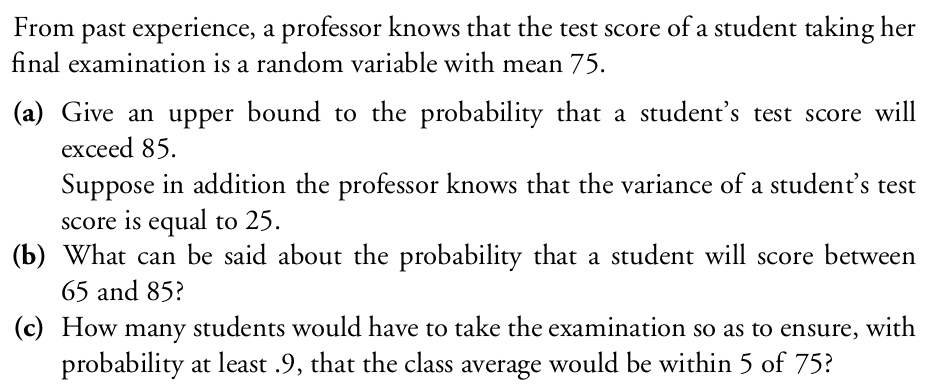
(a) By Markov inequality, $E(X)\geq 85 P(X> 85).$
So $P(X> 85) \leq \frac{75}{85}.$
(b) $P(65\leq X \leq 85) =
P(|X-75|\leq 10) = 1- P(|X-75|> 10)\geq 1-\frac{V(X)}{100} = \frac 34$ by Chebyshev.
(c) Let the answer be $n$, and class average be $\bar X.$
Then $E(\bar X) = 75$ and $V(\bar X) = \frac{25}{n}.$
So, by the Chebyshev inequality, $P(|\bar X-75|\geq 5) \leq \frac{25}{5^2n} = \frac 1n. $
So we need $1-\frac 1n \geq 0.9$ or $n\geq 10.$
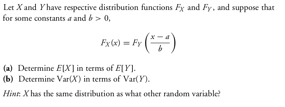
Here $P(X\leq x) = F_X(x) = F_Y\left(\frac{x-a}{b}\right) = P\left(Y\leq \frac{x-a}{b}\right) = P(a+bY\leq x).$
Since this holds for all $x\in{\mathbb R},$ hence $X$ and $a+bY$ have the same CDF.
Since $CDF$ is unique for a distribution, hence $X$ and $a+bY$ have the same distribution.
(a) $E(X) = E(a+bY) = a+bE(Y).$
(b) $V(X) = V(a+bY) = b^2 V(Y).$