 |
|---|
| Last updated on: Wed Jul 29 13:25:01 IST 2026 |
EXAMPLE 1: Roll a fair die. Let the outcome be denoted by $\omega.$ Define the random variables $X$ and $Y$ as
EXAMPLE 2: Roll a fair die and a fair coin independently together. Let the outcome be denoted by $\omega\equiv(\omega_1,\omega_2),$ where $\omega_1$ is the outcome of the die, and $\omega_2$ is that of the coin.
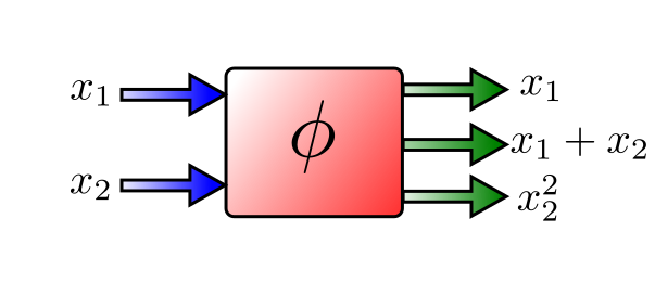
Define the random variables $X$, $Y$ and $Z$ asEXAMPLE 3: $\phi(x_1,x_2) = (x_1,x_1+x_2,x_2^2)$ is one such example. Here $\phi:{\mathbb R}^2\rightarrow{\mathbb R}^3.$ It has two inputs and 3 outputs:
|
|---|
EXAMPLE 4: The $\phi$ from the last example has component functions $$\phi_1(x_1,x_2) = x_1,~~ \phi_2(x_1,x_2) = x_1+x_2\mbox{ and } \phi_3(x_1,x_2) = x_2^2.$$ Note that, as in the case of the first and third components, not all the input variables need to appear in all the components. ■
EXAMPLE 5: Let $\phi:{\mathbb R}^2\rightarrow{\mathbb R}^2$ be $\phi(x_1,x_2) = (\sin (x_1x_2),\, x_1-x_2^2).$ Find its Jacobian. Also find the determinant of the Jacobian.
SOLUTION: The component functions are $\phi_1(x_1,x_2) = \sin(x_1x_2)$ and $\phi_2(x_1,x_2) = x_1-x_2^2.$ In our case $$\begin{eqnarray*} \frac{\partial \phi_1}{\partial x_1} & = & x_2\cos (x_1x_2),\\ \frac{\partial \phi_1}{\partial x_2} & = & x_1\cos (x_1x_2),\\ \frac{\partial \phi_2}{\partial x_1} & = & 1\\ \frac{\partial \phi_2}{\partial x_2} & = & -2x_2. \end{eqnarray*}$$ So the Jacobian is $$\left[\begin{array}{ccccccccccc}x_2\cos (x_1x_2) & x_1\cos (x_1x_2)\\ 1 & -2x_2 \end{array}\right].$$ Its determinant is $$x_2\cos (x_1x_2)\times(-2x_2)- x_1\cos (x_1x_2)\times 1 = -(2x_2^2+x_1)\cos (x_1x_2).$$ ■EXERCISE 1: Consider the random vector $(X,Y)$, where $X,Y$ are iid $N(0,1)$ random variables. If we generate a random sample of size 100 of this random variable, how will the scatterplot look like?
EXERCISE 2: Consider the random vector $(X,X)$, where $X$ is a $N(0,1)$ random variable. If we generate a random sample of size 100 of this random vector, how will the scatterplot look like?
EXERCISE 3: How many component functions does $\phi:{\mathbb R}^6\rightarrow{\mathbb R}^2$ have? $6?$ or $2?$
EXERCISE 4: Find the Jacobian of $\phi(x_1,x_2) = (x_1,x_1+x_2,x_1^2)$
EXERCISE 5: Compute the Jacobian matrix for $\phi(x,y,z) = (\sin(2x+3y),x^2z).$
EXERCISE 6: What is the Jacobian matrix for the transform $\phi:{\mathbb R}^n\rightarrow{\mathbb R}^n$ where $\phi(\v x) = A\v x+\v b$ for some fixed matrix $A_{n\times n}$ and fixed vector $\v b_{n\times 1}$?
EXERCISE 7: If $\phi:{\mathbb R}^n\rightarrow{\mathbb R}^n$ is given by $\phi(\v x) = A\v x+\v b$ for some matrix $A_{n\times n}$ and vector $\v b_{n\times 1}$, then show that $\phi$ is one-one if and only if $A$ is nonsingular.
EXERCISE 8: If $\phi:{\mathbb R}^2\rightarrow{\mathbb R}^2$ is a one-one function, then must both its component functions also be one-one?
EXERCISE 9: If $\phi:{\mathbb R}^2\rightarrow{\mathbb R}^2$ has one-one component functions, then must $\phi$ itself also be one-one?
EXAMPLE 6: Let $X$ have exponential distribution with rate $\lambda>0.$ Find the density of $X^2.$
SOLUTION: Here $X$ has density $f(x) = \left\{\begin{array}{ll} \lambda e^{-\lambda x}&\text{if }x > 0\\ 0&\text{otherwise.}\end{array}\right..$ Also $\phi:(0,\infty)\rightarrow(0,\infty)$ is a bijection, with differentiable $\phi ^{-1}(y) = \sqrt y.$ So $X^2$ has density $$\begin{eqnarray*} g(y) & = & f(\phi ^{-1}(y)) \left| \frac{d\phi ^{-1}(y)}{dy} \right|\\ & = & \left\{\begin{array}{ll}\lambda e^{-\lambda\sqrt y} \left| \frac{1}{2\sqrt y} \right|&\text{if }y>0\\ 0&\text{otherwise.}\end{array}\right.\\ & = & \left\{\begin{array}{ll}\frac{ \lambda e^{-\lambda\sqrt y}}{2\sqrt y} &\text{if }y>0\\ 0&\text{otherwise.}\end{array}\right.. \end{eqnarray*}$$ You may check the statistical regularity behind this exercise by direct simulation. In the following snippet I have used $\lambda=2.$
g = function(y) {exp(-2*sqrt(y))/sqrt(y)}
x = rexp(1000,rate=2)
hist(x^2,prob=T)
curve(g,add=T)
■
EXERCISE 10: If $X$ has exponential distribution with rate $\lambda>0,$ find the density of $\log X.$
EXERCISE 11: If $X\sim Unif(0,1)$ then what is the density of $\cos X$?
EXERCISE 12: If $X$ has density $f(x),$ and $a(\neq0),b\in{\mathbb R}$ are fixed, then find the density of $aX+b.$
EXERCISE 13: If $X\sim Unif\left(-\frac \pi2,\frac \pi2\right),$ find the density of $\tan X.$
EXAMPLE 7: Let $\v X = (X_1,X_2)$ be uniformly distributed over $[1,2]\times[3,4].$ Let $Y_1 = X_1X_2$ and $Y_2 = X_1.$ Find the joint density of $\v Y = (Y_1,Y_2).$
SOLUTION: Let $S = [1,2]\times[3,4].$ This has area 1. So $\v X $ has density $$f(x_1,x_2) = \left\{\begin{array}{ll}1&\text{if }(x_1,x_2)\in S\\ 0&\text{otherwise.}\end{array}\right..$$ Here the transform is $\phi(x_1,x_2) = (x_1x_2,x_1).$ Clearly, $\phi:S\rightarrow \phi(S)$ is one-one, because given $y_1=x_1x_2$ and $y_2=x_1$ you can recover $(x_1,x_2)\in[1,2]\times[3,4]$ uniquely as $x_1 = y_2$ and $x_2 = \frac{y_1}{y_2}.$ Thus, the inverse transform is $\phi ^{-1}(y_1,y_2) = \left(y_2,\frac{y_1}{y_2}\right).$ The Jacobian of this is $$\left[\begin{array}{ccccccccccc}0 & 1\\\frac{1}{y_2} & -\frac{y_1}{y_2^2} \end{array}\right],$$ which has absolute determinant $\frac{1}{y_2},$ since $y_2 > 0.$ So the required density will be $$g(y_1,y_2) = \left\{\begin{array}{ll}\frac{1}{y_2}&\text{if }\left(y_2,\frac{y_1}{y_2}\right)\in S\\ 0&\text{otherwise.}\end{array}\right.$$ Often we want to write it as $$g(y_1,y_2) = \left\{\begin{array}{ll}\frac{1}{y_2}&\text{if }(y_1,y_2)\in \phi(S)\\ 0&\text{otherwise.}\end{array}\right.$$ To find out $\phi(S)$ remember that $\v x\in S\Leftrightarrow \v y\in \phi(S).$ We shall start with $\v x\in S,$ i.e., $\phi ^{-1}(\v y)\in S,$ which, in our example, is $\left(y_2,\frac{y_1}{y_2}\right)\in S.$ This means $$1\leq y_2 \leq 2 \mbox{ and } 3\leq \frac{y_1}{y_2}\leq 4.$$ Sketching these restrictions we get this region: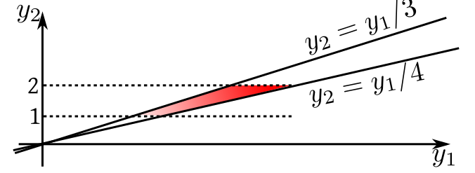 |
|---|
| $\phi(S)$ shown in red |
EXERCISE 14: If $(X_1,X_2)$ has joint density $f(x)=\left\{\begin{array}{ll}x_1+x_2&\text{if }x_1,x_2\in[0,1]\\ 0&\text{otherwise.}\end{array}\right.$, then find the joint density of $(X_1+X_2, X_1-X_2).$
EXERCISE 15: If $(X_1,X_2)$ is uniformly distributed over $[0,1]\times[0,2]$, then find the joint density of $(X_1^2,X_1+X_2).$
EXERCISE 16: If $X_1,X_2$ are iid $N(0,1)$ random variables, and $(R,\Theta)$ is the polar representation of $(X_1,X_2),$ then find the density of $(R,\Theta).$
EXERCISE 17: If $X_1,X_2$ are iid exponential random variables with rate 1, and $(R,\Theta)$ is the polar representation of $(X_1,X_2),$ then find the density of $(R,\Theta).$
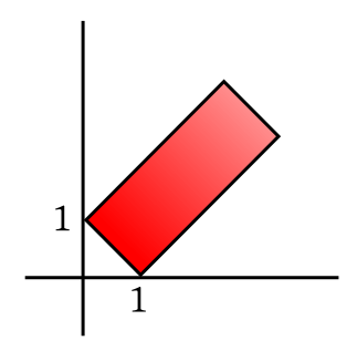
EXERCISE 18: If $(X_1,X_2)$ is uniformly distributed over the red rectangle below, then find non-zero constants $a,b,c,d$ such that $Y_1=aX_1+bX_2$ and $Y_2=cX_1+dX_2$ are independent.
 |
|---|
Hint:
The answer is not unique.
EXERCISE 19: Let $(X_1,X_2)\sim Unif([0,1]\times[0,2]).$ Find the joint density of $(Y_1,Y_2),$ where $Y_1 = X_1+2X_2+1$, $Y_2 = 3X_1+X_2.$
EXERCISE 20: If $(X_1,X_2)$ has joint density $f(x_1,x_2) = \left\{\begin{array}{ll}x_1+x_2&\text{if }x_1,x_2\in[0,1]\\ 0&\text{otherwise.}\end{array}\right.,$ then find the joint density of $(X_1+X_2,X_2).$
EXERCISE 21: If $X_1,X_2$ are iid Cauchy, then find the joint density of $((X_1+X_2)/2, X_1+1).$
EXERCISE 22: If $X_1,X_2,X_3$ are iid $N(0,1)$ random variables, Find the joint density of $A\left[\begin{array}{ccccccccccc}X_1\\X_2\\X_3 \end{array}\right]$ where $A$ is some fixed nonsingular matrix and $\v b$ is some fixed vector.
Hint:
The joint density of $\v X = \left[\begin{array}{ccccccccccc}X_1\\X_2\\X_3 \end{array}\right]$ is $$f(\v x) = (2\pi)^{-\frac 32} \exp\left(-\frac 12\v x' \v x\right)\mbox{ for } \v x\in{\mathbb R}^3.$$
Let $(X_1,X_2)$ have joint density $f(x_1,x_2).$ Then the (marginal) density of $X_1$ is $f_{X_1}(x_1) = \int_{-\infty}^\infty f(x_1,x_2)\, dx_2.$In other words, you can "integrate out" the unwanted variables. This works in higher dimensions also, as shown in the example below.
EXAMPLE 8: Let $(X_1,X_2,X_3,X_4)$ have joint density $f(x_1,x_2,x_3,x_4).$ How would you find the density of $(X_1,X_3)?$
SOLUTION: It is $f_{X_1,X_3}(x_1,x_3) = \int_{-\infty}^\infty\int_{-\infty}^\infty f(x_1,x_2,x_3,x_4)\, dx_2dx_4.$ This integral may look complicated. But in order to evaluate it, just perform two integrations, once wrt $x_2$ and once wrt $x_4$ (each time considering all other $x_i$'s as constants). You may perform the two integrations in any order you like. ■ Here is a more numerical example.EXAMPLE 9: If $(X_1,X_2)$ has joint density $$f(x_1,x_2) = \left\{\begin{array}{ll}2(x_1 + x_2)&\text{if }x_1\in[0,1], x_2\in[0,x_1]\\ 0&\text{otherwise.}\end{array}\right.,$$ then find the (marginal) density of $X_1.$
SOLUTION: Let's start by sketching the support of the joint density: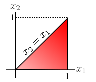 |
|---|
| The red triangle is where the density is positive. |
EXERCISE 23: Work out the (marginal) density of $X_2$ in the example above.
EXERCISE 24: Let $(X_1,X_2)$ have joint density $$f(x_1,x_2) = \left\{\begin{array}{ll}24x_1x_2&\text{if }x_1,x_2\geq 0\mbox{ and }x_1+x_2\leq 1\\ 0&\text{otherwise.}\end{array}\right..$$ Find the (marginal) density of $X_1.$ Don't forget to sketch the support first!
EXERCISE 25: Find the density of $X_2$ for the joint density in the exercise above.
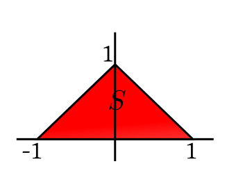
EXERCISE 26: Let $(X_1,X_2)$ be distributed uniformly over the set $S$ shown below.
 |
|---|
EXAMPLE 10: Let the joint density of $(X,Y)$ be $$f(x,y)=\left\{\begin{array}{ll}x+y&\text{if }0\leq x,y\leq 1\\ 0&\text{otherwise.}\end{array}\right..$$ Find the joint density of $2X+3Y.$
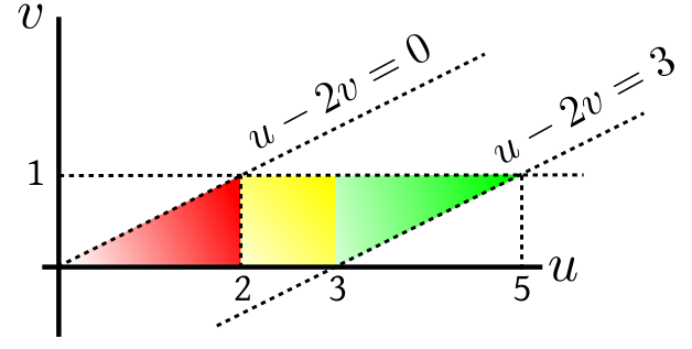
SOLUTION: Here the function is $\phi_1(x,y) = 2x+3y.$ Since the codomain is ${\mathbb R},$ we make it ${\mathbb R}^2$ by padding it with another function of our choice, say $\phi_2(x,y) = x.$ Then the padded function is $\phi(x,y)\mapsto (2x+3y,x).$ This is a one-one function from ${\mathbb R}^2$ to ${\mathbb R}^2.$ Taking $(u,v) = (2x+3y,x)$ the inverse transform is $(x,y) = \left(v,\frac{u-2v}{3}\right),$ with Jacobian $\left[\begin{array}{ccccccccccc}0 & 1\\\frac 13 & -\frac 23 \end{array}\right].$ Its absolute determinant is $\frac 13.$ So the joint density of $(U,V)$ is $$g(u,v) = \frac 13f\left(v,\frac{u-2v}{3}\right) =\left\{\begin{array}{ll}\frac{u+v}{9}&\text{if }0\leq v,\frac{u-2v}{3}\leq 1\\ 0&\text{otherwise.}\end{array}\right..$$ In other words, $$g(u,v) =\left\{\begin{array}{ll}\frac{u+v}{9}&\text{if }(u,v)\in \phi(S)\\ 0&\text{otherwise.}\end{array}\right.,$$ where $\phi(S)$ is the red region below.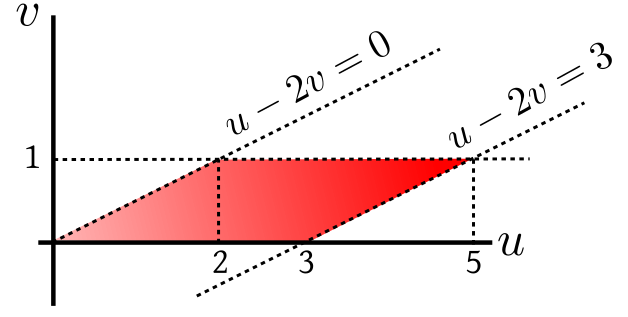 |
|---|
 |
|---|
| The three parts |
EXERCISE 27: Let $(X,Y)$ have joint density $f(x,y).$ Find the density of $X+Y$ by "padding" it up with $X.$
EXERCISE 28: Let $(X,Y)$ have joint density $f(x,y).$ Find the density of $X+Y$ by "padding" it up with $Y.$ Did you get the same answer as in the exercise above?
EXERCISE 29: Let $X,Y$ be iid Cauchy random variables. Find density of $\frac{X+Y}{2}.$
EXERCISE 30: Let $(X,Y)$ have joint density $f(x,y).$ Find the density of $X-Y.$
EXERCISE 31: Let $(X,Y)$ have uniform density over $[1,2]\times[3,4].$ Find the density of $XY.$
EXERCISE 32: Let $X,Y$ be iid exponential random variables with rate $1.$ Find density of $\frac XY.$
 |
|---|
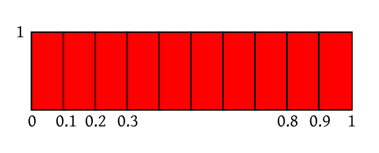
| All the rectangles are identical |
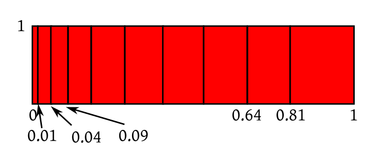 |
|---|
| The subintervals are scaled non-uniformly |
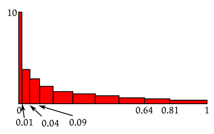 |
|---|
| All rectangles now again have area $\frac{1}{10}.$ |
EXERCISE 33: If $X$ has uniform distribution over (2,4) then roughly sketch the density of $Y = \frac 1X.$ Don't apply the Jacobian formula algeraically. Think in terms of which part gets squeezed/expanded.
EXERCISE 34: Suppose that $X$ is uniform over $(-1,1)$ and $Y=X^2.$ (not a bijection!). Guess the form of the density of $Y.$ Do you see why we needed the transform to be bijective in our intuition?
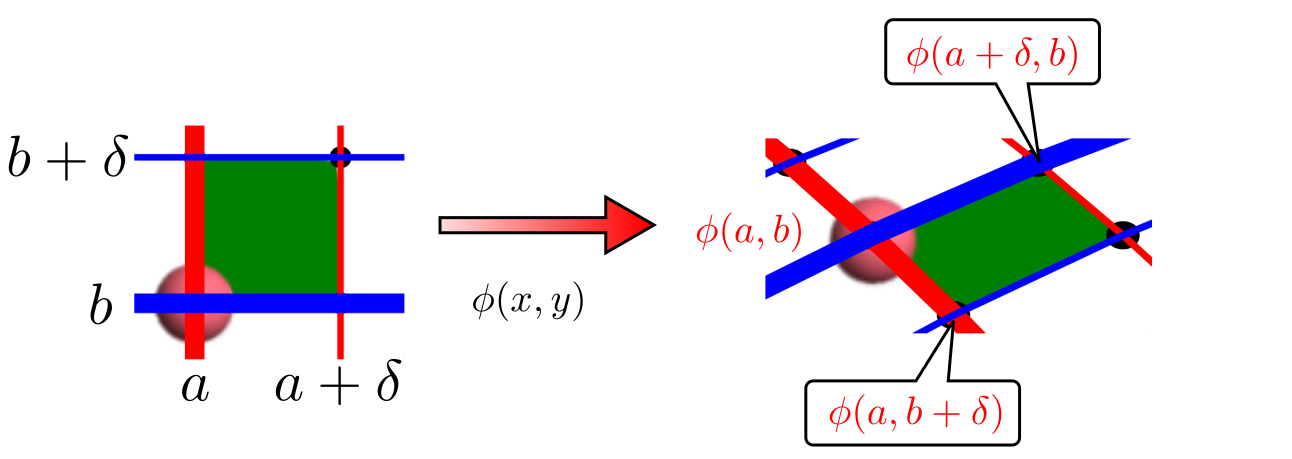
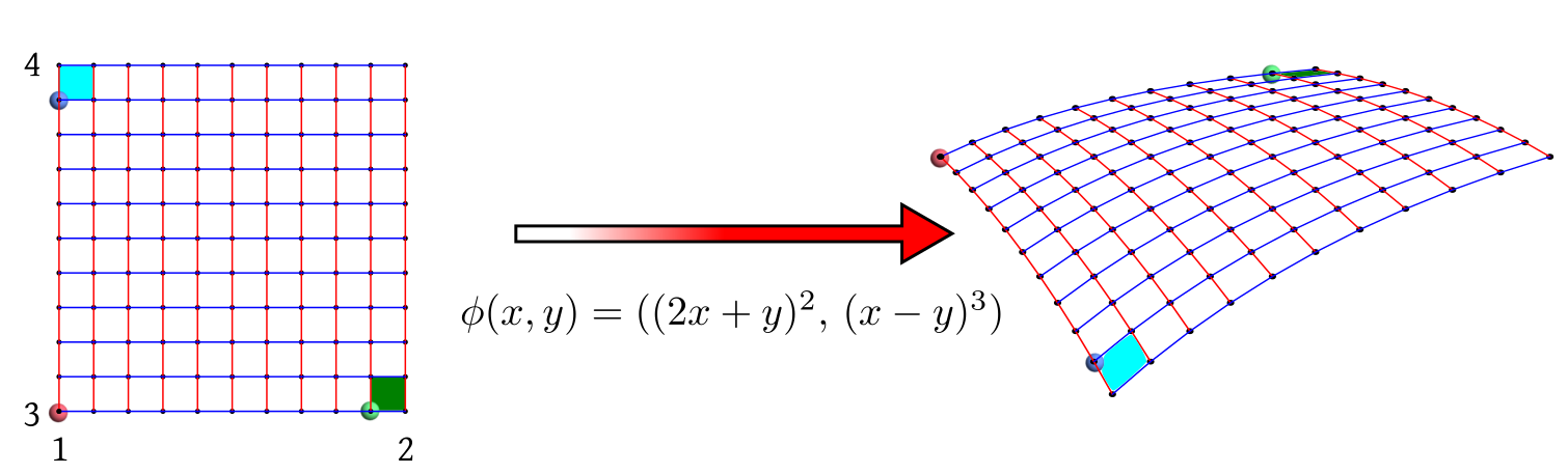 |
|---|
| A transform from ${\mathbb R}^2$ to ${\mathbb R}^2$ |
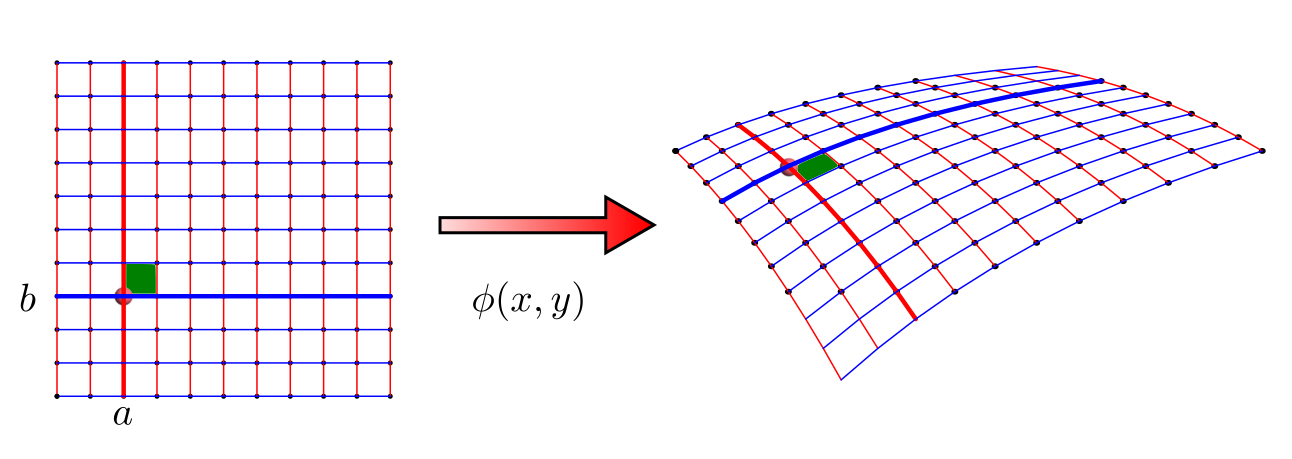 |
|---|
| Notice how the little green square changes |
 |
|---|
| A closer look |
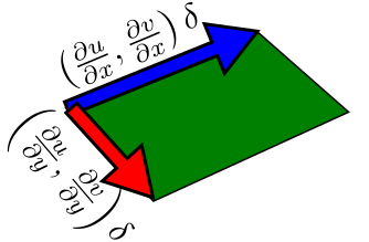 |
|---|
| A parallelogram |
EXERCISE 35: Consider the transformation $\phi(x,y) = (x,2y).$ Sketch how a square $[a,a+\delta]\times[b,b+\delta]$ is transformed by it. By what factor does the area grow? Answer this both from your diagram as well as Jacobian determinant.
EXERCISE 36: Consider the transformation $\phi(x,y) = (x,-2y).$ Sketch how a square $[a,a+\delta]\times[b,b+\delta]$ is transformed by it. By what factor does the area grow? Answer this both from your diagram as well as Jacobian determinant.
EXERCISE 37: Consider the transformation $\phi(x,y) = (2x,3y).$ Sketch how a square $[a,a+\delta]\times[b,b+\delta]$ is transformed by it. By what factor does the area grow? Answer this both from your diagram as well as Jacobian determinant.
EXERCISE 38: Consider the transformation $\phi(x,y) = (x^3,y^3).$ Which point in the region $[1,2]\times[3,4]$ experiences the maximum stretch?