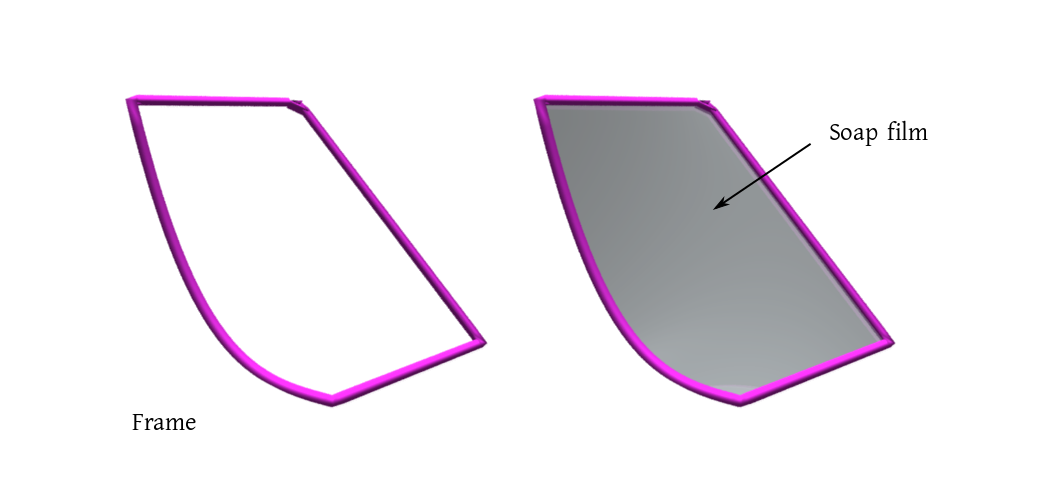
If you dip a wire frame in a soap solution, then a thin film of soap water
will cling to it.
Given the shape of the frame, we want to find the natural shape of the film. This is an important
question in architecture, where a structure must be given the most
natural shape to reduce stress.
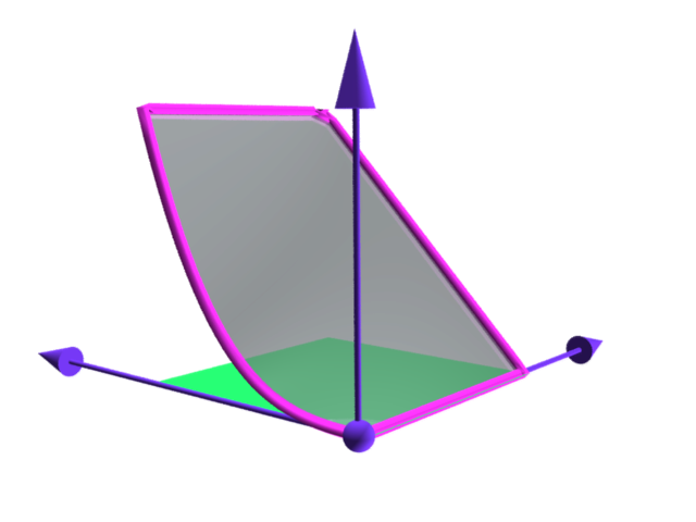
It is known that a soap film will always occupy the position that
minimises its elastic potential energy. In the next section we
shall see how to express this mathematically.
If the surface is given by a function $u(x,y),$ then its
elastic potential energy is given by
$$
E(u) = \iint_R (u_x)^2 + (u_y)^2\, dxdy.
$$
This is to be minimised subject to the boundary condition that
the $u(x,y)$ must match the frame height at the boundary.
In general, this is a difficult/impossible problem to solve
analytically.
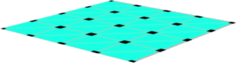
To proceed numerically, one starts with a
triangulation of the base.
Triangulation
Then the aim is to find the value of $u(x,y)$ at the
vertices. Let $c_j$ denote the value of $u(x,y)$ at the
$j$-th vertex.
Since the target function involves $u_x$
and $u_y$, we need to somehow approximate them using only
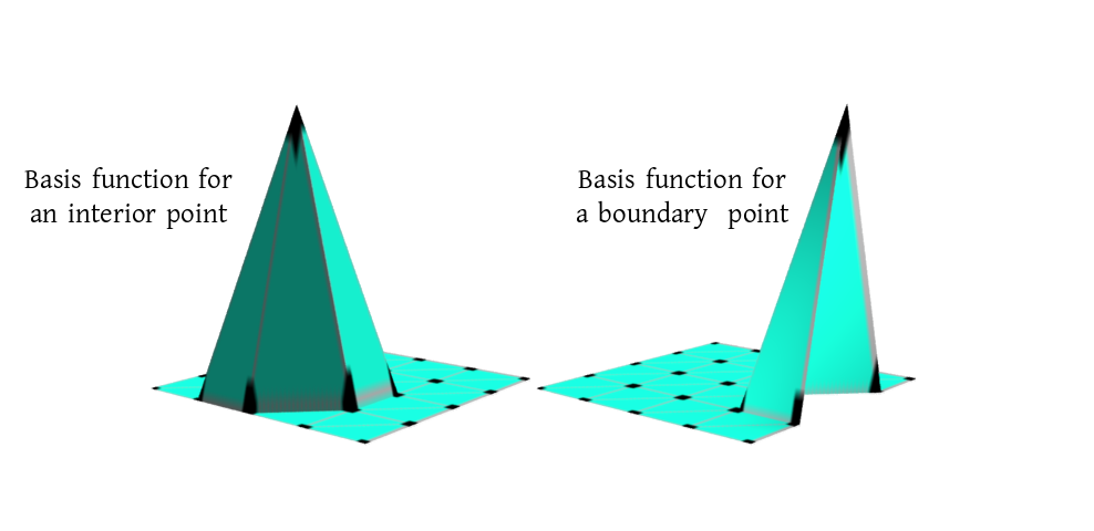
the values at the vertices. For this we choose a set of basis
functions, one for each vertex. It is constructed by "pulling
up" the vertex to a height 1, while leaving all the other
vertices at height 0. Here are two examples:
Two basis functions
Notice that the graph of each basis function ($\phi_j$) is a plane over
each triangle ($T_i$). and hence we may write a basis
function $\phi_j(x,y)$ as
$$
\phi_j(x,y) = \alpha_{ij} + \beta_{ij}x + \gamma_{ij} y \quad\mbox{
for } (x,y)\in T_i.
$$
for suitable numbers $\alpha_{ij},$ $\beta_{ij}$
and $\gamma_{ij}$.
Also, notice that $\alpha_{ij}, \beta_{ij},
\gamma_{ij}$'s are zero if the $j$-th vertex is not part
of $T_i$. Thus, most of these numbers are actually zero.
Then we can approximate $u(x,y)$ by
$$
u(x,y) = \sum_j c_j \phi_j(x,y).
$$
Thus, the problem of finding $u(x,y)$ reduces to finding the
finitely many numbers $c_j$'s.
Now
$$
u_x(x,y) = \sum_j c_j\beta_{ij} \mbox{ for } (x,y)\in T_i^\circ,
$$
where $T_j^\circ$ denotes the interior of $T_j.$
Similarly for $u_y(x,y).$
Hence we have
$$
E(u) = \sum_i \iint_{T_i^\circ} (\sum_j c_j \beta_{ij})^2 + (\sum_j c_j\gamma_{ij})^2
= \sum_i |T_i| \{ (\sum_j c_j \beta_{ij})^2 + (\sum_j c_j\gamma_{ij})^2 \},
$$
where $|T_i|$ denotes the area of $T_i$ (same as the
area of $T_i^\circ$).
Thus,
$$
E(u) = \bc' M\bc,
$$
where $M$ is the NND matrix with $(j,j')$-th entry given
by
$$
m_{jj'} = \sum_i |T_i| (\beta_{ij}\beta_{ij'} + \gamma_{ij} \gamma_{ij'}).
$$
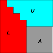
Suppose that the last $k$ of the $c_j$'s are
known frame heights. Partition $\bc$
as $(\bc_1,\bc_2).$ Then $\bc_2$ is known,
and $\bc_1$ is to be chosen to minimise $E(u).$
Let us partition $M$ accordingly as
$$
M = \left[\begin{array}{ccccccccccc}M_{11} & M_{12}\\M_{21} & M_{22}
\end{array}\right].
$$
Then
$$
\bc' M\bc = \left[\begin{array}{ccccccccccc}\bc_1' & \bc_2'
\end{array}\right]\left[\begin{array}{ccccccccccc}M_{11} &
M_{12}\\M_{21} & M_{22}
\end{array}\right] \left[\begin{array}{ccccccccccc}\bc_1\\\bc_2
\end{array}\right] =
\bc_1' M_{11}\bc_1 + 2\bc_1' M_{12}\bc_2 + \bc_2' M_{11}\bc_2.
$$
Differentiating w.r.t. $\bc_1$, and equating to zero, we get
$$
M_{11}\bc_1 + M_{12}\bc_2 = \bz,
$$
or
$$
M_{11}\bc_1 = - M_{12} \bc_2.
$$
Here is a quick primer
of multivariate differentiation, in case you need one.
It is a simple linear algebra exercise to show that this is
always consistent. In fact, $M_{11}$ will also be
nonsingular (not easy to prove). So the problem always has unique solution.
However,
there is a practical difficulty. To get a reasonable
approximation we need the number of vertices to be pretty
large. In our example, the vertices are in a rectangular array formed
by subdividing the sides of the base. If we use 100 subdivisions
in both directions, then the number of vertices is $101^2,$
of which $99^2=9801$ are interior vertices. Thus, we need to
solve $9801$ equations in as many unknowns! For many real
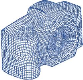
life problem we need even more vertices:
Many vertices are needed to capture the
nooks and corners.
However, notice that $M_{11}$ is an extremely sparse
matrix. Each row contains just 6 nonzero entries. Using
Gauss-Jordan elimination is not a good idea in such a case, as it
destroys the sparseness of the system. There are special
algorithms for such cases that we shall learn now.
Gauss and Gauss-Jordan elimination suffer from one problem:
accumulation of errors. If the system is large then the solution obtained
by these methods is usually not as precise as can be desired. Remember
that due to finite precision of the computer some error is always
inevitable. But the the solution obtained by Gauss or Gauss-Jordan
eliminations often produce error larger than the minimum error possible
with the machine. In such situation one may try to improve the precision of
the solution by applying iterative methods like the one discussed
below. However, this is not the most popular reason for the using
iterative methods.
A more compelling reason to use these methods is when the system is
sparse. A sparse system is where many of the entries of the
coefficient matrix are known to be zero. Such matrices occur in
different applications. Gauss and Gauss-Jordan eliminations cannot take
advantage of the zeros. The iterative methods on the other hand work faster
for sparse matrices.
Consider a linear system of equations
$$
A\bx={\bf b},
$$
where $A$ is a square matrix.
EXAMPLE:
Suppose that you are to solve
$$\begin{eqnarray*}
20x+3y-4z & =& 19\\
x-4y+z & =& -3\\
x-4y+10z & =& 7.
\end{eqnarray*}$$
The system has three equations in three unknowns. To solve it by
Gauss-Jacobi method we solve for $x$ in the first equation, for
$y$ in the second equation and so on. Solving for $x$ in the
first equation means keeping $x$ in the left hand side and taking
everything else to the right hand side:
$$
x = (19-3y+4z)/20.
$$
Similarly, we get three equations by solving for $x,y,$ and $z$
from the three equations:
$$\begin{eqnarray*}
x & =& (19-3y+4z)/20\\
y & =& (3+x+z)/4\\
z & =& (7-x+4y)/10.
\end{eqnarray*}$$
Now take any three numbers
$x_0,y_0$ and $z_0$
as initial guesses for $x,y$and $z.$ Suppose that we take
$$
\left[\begin{array}{ccccccccccc}x_0\\y_0\\z_0
\end{array}\right] = \left[\begin{array}{ccccccccccc}0\\0\\0
\end{array}\right].
$$
Use these in the right hand sides of the three equations, to compute
$x_1,y_1,z_1.$ Thus,
$$
\left[\begin{array}{ccccccccccc}x_1\\y_1\\z_1
\end{array}\right] = \left[\begin{array}{ccccccccccc}(19-3y_0+4z_0)/20\\
(3+x_0+z_0)/4\\
(7-x_0+4y_0)/10
\end{array}\right] = \left[\begin{array}{ccccccccccc}0.9500\\0.7500\\0.7000
\end{array}\right].
$$
Similarly, we get $x_2,y_2,z_2$ from $x_1,y_1,z_1,$ and so
on. We show the values of $x_i,y_i,z_i$ for $i=0,1,...,5:$
Thus, after 10 iterations our answer is given by the last row.
This is called the Gauss-Jacobi method.
How accurate is this answer? To check this let us compute
$$
A\bx-{\bf b}.
$$
Ideally, it should be the zero vector. For our answer it turns out to be
$$
\left[\begin{array}{ccccccccccc}-0.000002\\0.000002\\-0.000007
\end{array}\right],
$$
which is quite close to zero.
EXAMPLE:
Let us consider the same system of
equation once again. As before, we shall solve for $x$ from the first
equation, for $y$ from the second equation, and so on. Thus, we
arrive at the three equations (as before):
$$\begin{eqnarray*}
x & =& (19-3y+4z)/20\\
y & =& (3+x+z)/4\\
z & =& (7-x+4y)/10.
\end{eqnarray*}$$
Again, start with, say,
$$
\left[\begin{array}{ccccccccccc}x_0\\y_0\\z_0
\end{array}\right] = \left[\begin{array}{ccccccccccc}0\\0\\0
\end{array}\right].
$$
But this time, apply the equations one by one. Thus, we first
compute $x_1$ as
$$
x_1 = (19-3y_0+4z_0)/20 = 0.95.
$$
Then we compute $y_1$ using this $x_1$
$$
y_1 = (3+x_1+z_0)/4 = 0.9875.
$$
Observe that we are using $x_1$ and $z_0$ in the right hand side.
This is the only difference between between the Gauss-Seidel and
Gauss-Jacobi method. In Gauss-Seidel method we always use the most recent
value available. Thus, to compute $z_1$ we shall use the most recent
values of $x$ and $y,$ namely, $x_1$ and $y_1:$
$$
z_1 = (7-x_1+4y_1)/10.
$$
Then we shall compute $x_2$ from $y_1,z_1.$ After that we shall
compute $y_2$ from $x_2,z_1,$ and so on. We show the values of
$x_i,y_i,z_i$ in the following table for $i=0,1,...,10.$
The following discussion involves some advanced techniques, and
I have skipped the proofs of the some of the results. For a
comprehensive discussion see the book Matrix Computations
by Golub and Van Loan.
Both these methods are special cases of splitting methods, where
a nonsingular system
$$
A\bx = \bb
$$
is written as
$$
M\bx = N\bx + \bb.
$$
Here $A$ is split as $M-N$ with $M$ nonsingular. Then
$$
\bx = M^{-1} N \bx + M^{-1}\bb.
$$
We use the iteration
$$
\bx_{n+1} = M^{-1} N \bx_n + M^{-1}\bb.
$$
EXAMPLE:
In Gauss-Jacobi $M$ consists of the diagonal elements
of $A.$
EXERCISE:
What is $M$ in the Gauss-Seidel method?
Let the actual solution be $\bxi = A^{-1}\bb.$ Then
$$
\bxi = M^{-1} N \bxi + M^{-1}\bb.
$$
Subtracting this from the last equation we get
$$
\bx_{n+1}-\bxi = M ^{-1} N (\bx_n-\bxi),
$$
or
$$\be_{n+1} = M^{-1} N \be_n,$$
where $\be_n = \bx_n-\bxi$ is the error committed in step $n$.
We need some condition of $M ^{-1} N$ for the
sequence $(\be_n)$ to converge to $\bz.$
A necessary and sufficient condition is based on the following
definition.
This is not very easy to prove. In fact, even checking that the
spectral radius is $< 1$ is not easy. We shall discuss two
sufficient condtions for this: strict diagonal dominance in case
of Gauss-Jacobi, and
positive definiteness in case of Gauss-Seidel.
EXAMPLE:
The following matrix has strict diagonal dominance property:
$$
\left[\begin{array}{ccccccccccc}10& 1& -5\\-1& 3& 1\\1& 3& 20
\end{array}\right].
$$
However the matrix below does not have the property.
$$
\left[\begin{array}{ccccccccccc}1& 2& -3\\2& 14& 3\\3& 4& 10
\end{array}\right],
$$
since in the first row
$$
1 \not > 2+|-3|.
$$
Proof:
Enough to show that the spectral radius of $C=M^{-1}N$ is $<1.$
Here the $(i,j)$-th element of $C$ is
$$
c_{ij} = \left\{\begin{array}{ll}
-\frac{a_{ij}}{a_{ii}} &\text{if }i\neq j\\
0 &\text{otherwise.}
\end{array}\right.
$$
Thus $\forall i~~\sum_j |c_{ij}| < 1.$
This implies that all the eigen values of $C$ must
have moduli $< 1.$
Because:
Let $\lambda$ be an eigen value
of $C,$ and let $\bv$ be a corresponding
eigen vector.
Let the $k$-th entry of $\bv$ have max modulus:
$$
\forall i~~|v_k| \geq |v_i|.
$$
Then consider the $k$-th row of $\lambda\bv = C\bv$
to have
$$
\lambda v_k= \sum_j c_{kj} v_j,
$$
or,
$$
|\lambda| |v_k|\leq \sum_j |c_{kj}| |v_j| \leq |v_k|\sum_j
|c_{kj}|,
$$
or
$$
|\lambda| \leq \sum_j|c_{kj}| < 1.
$$
So spectral radius of $C$ must be $<1,$ as well.
[QED]
Proof:
Here the coefficient matrix can be written as
$$
A = L + D + L',
$$
where $L$ is the strict lower triangular half, $D$ is
the diagonal part (and so $L'$ is the strict upper
triangular half). Then the Gauss-Seidel method uses the splitting
$A = M - N$, where
$$
M = L+D\mbox{ and } N = -L'.
$$
So enough to show that $C = M ^{-1} N = -(L+D)^{-1}L'$ has
spectral radius $<1,$ i.e, all eigen values of $C$
has moduli $< 1.$
Now eigen values of $C$ are the same as the eigen values of
$$\begin{eqnarray*}
C_1
& =& D^{1/2}CD^{-1/2} \\
& =& -D^{1/2}(L+D)^{-1}L'D^{-1/2}\\
& = &
-D^{1/2}(L+D)^{-1}D^{1/2}D^{-1/2}L'D^{-1/2}\\
& = &
-(I + L_1)^{-1} L_1',
\end{eqnarray*}$$
where $L_1=D^{-1/2}LD^{-1/2}.$
Notice that though $C_1$ is similar to $C,$
but $L_1$ may not be similar to $L.$
Now let $\lambda$ be any eigen
value of $C_1.$ Take any eigen vector $\bx$ with
$\bx^*\bx=1.$
Then $C_1\bx = \lambda \bx,$ i.e., $-(I + L_1)^{-1}
L_1'\bx = \lambda \bx,$ or
$$
-L_1'\bx = \lambda(I+L_1)\bx,
$$
and so
$$
-\bx^*L_1'\bx = \lambda\bx^*(I+L_1)\bx = \lambda(1+\bx^*L_1\bx).
$$
Let $z=\bx^*L_1\bx.$ Then $\bx^*L_1'\bx=\zbar.$
So we have
$$
-\zbar = \lambda(1+z).
$$
Hence
$$
|\lambda| = \frac{|z|}{|1+z|} = \frac{ |z-0| }{ |z-(-1)| }.
$$
We are to show that $|\lambda|<1,$ i.e., $z$ is closer
to $0$ than to $-1$ in the complex plane.
Now notice that
$$
I + L_1+L_1' = D^{-1/2} A D^{-1/2}
$$
is a p.d. matrix.
Because:$D^{-1/2}$ is a nonsingular
symmetric matrix, and for any nonsingular matrix $P$ the
matrix $P'AP$ must be p.d.
So
$$
\bx^*(I + L_1+L_1')\bx = 1+z+\zbar > 0.
$$
So $Re(z) > -\frac12,$ or $z$ is closer to 0 than
to $-1,$ completing the proof.
[QED]
The Gauss-Seidel and Gauss-Jacobi methods are special cases of a
class of methods called successive over relaxation (SOR)
method. Here we choose some $w>0$ and then write the
system $A\bx=\bb$ as $wA\bx=w\bb,$ and then
split $A$ into its diagonal and strict triangular halves
$$
A = L+D+U
$$
to get
$$
w(L+D+U)\bx = w\bb.
$$
We rearrange this to get the iterative scheme
$$
(D+wL)\bx_{n+1} = w\bb - (wU+(w-1)D)\bx_n.
$$
This system is easily solved by forward substitution
since $D+wL$ is lower triangular. Suitable choice
for $w$ (not always easy to obtain) speeds up convergence.
Find the natural shape of the soap film where
the base is the unit square, and the boundaries are the
graphs of the functions $0, $ $x,$ $1$
and $x^3.$ Use 50 subdivisions for each side.
[Hint: Don't worry. The final algorithm is very simple and intuitive!]
We say that a nonsingular matrix has $LU$ decomposition if it can be
written as
$$
A = LU,
$$
where $L$ is a lower triangular and $U$ is an upper triangular
matrix.
EXERCISE:
Show that such a factorization need not be unique even if one exists.
If $L$ has 1's on its diagonals then it is called Doolittle
decomposition and if $U$ has 1's on its diagonals, it is called
Crout's factorization. If $L = U'$ then we call it Cholesky
decomposition (read Cholesky as Kolesky.)
We shall work with Crout's decomposition as a representative $LU$
decomposition. The others are similar.
$LU$ decomposition is mainly used as a substitute for
matrix inversion. If $A=LU$ then you can
solve $A\bx=\bb$ as follows.
First write the system as two triangular systems
$$
L\by = \bb, \text{ where } \by = U\bx.
$$
Being triangular, the systems can be solved by forward or
backward substitution.
Apply forward substitution to solve for $\by$ from the first
equation, and then apply backward substitution to solve
for $\bx$ from the second equation.
Notice that, unlike Gaussian/Gauss-Jordan elimination, we do not
need to know $\bb$ while computing the $LU$
decomposition. This is useful when we want to solve many systems
of the form $A\bx=\bb$ where $A$ is always the same,
but $\bb$ will change later depending on the situation.
Then the $LU$ decomposition needs to be computed once and
for all. Only the two substitutions are to be done afresh for
each new $\bb.$
From definition of matrix
multiplication we have
$$
a_{ij} = \sum_{k=1}^n l_{ik} u_{kj}.
$$
Now, $l_{ik}=0$ if $k>i,$ and $u_{kj}=0$ if $k< j.$
So the above sum is effectively
$$
a_{ij} = \sum_{k=1}^{\min\{i,j\}} l_{ik} u_{kj}.
$$
You can compute $l_{i1}$ 's for $i\geq
1$ by considering
$$
a_{i1} = l_{i1}u_{11} = l_{i1},
$$
since diagonal entries of $U$ are 1. Once $l_{11}$ has been
computed you can compute $u_{1i}$'s for $i\geq
2$ by considering
$$
u_{1i} = a_{1i}/l_{11}.
$$
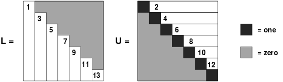
Next you will compute $l_{i2}$'s and after that $u_{2i}$'s, and
so on. The order in which you compute the $l_{ij}$'s and
$u_{ij}$'s is shown in the diagram below.
$LU$ decomposition computation order
The general formulas to compute $l_{ij}$ and $u_{ij}$ are
$$\begin{eqnarray*}
l_{ij} & = a_{ij} - \sum_{k=1}^{j-1}l_{ik} u_{kj}& (i\geq j)\\
u_{ij}& = \frac{1}{l_{ii}}\left(a_{ij} - \sum_{k=1}^{i-1}l_{ik}
u_{kj}\right)& (i< j).
\end{eqnarray*}$$
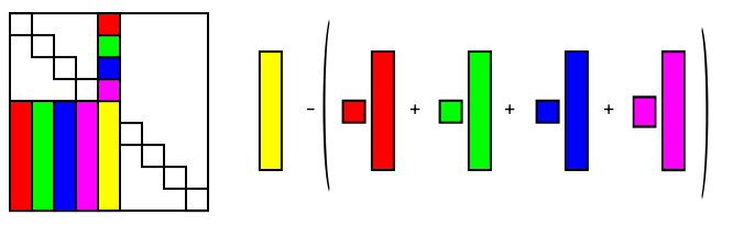
The following diagram might help to understand the computation of
the $l_{ij}$'s:
In order to compute the yellow part of $L,$ subtract a
linear combination from the yellow part of $A.$ The linear
combination is made of the corresponding parts of $L$
computed earlier, and the coefficients come from $U.$
This translates into the following R code:
L = function(j) {
  tot = rep(0,n-j+1)
  if(j>1) {
    for(k in 1:(j-1))
      tot = tot + A[j:n,k] * A[k, j]
  }
  A[j:n,j] <<- A[j:n,j] - tot
  A
}
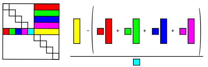
A similar diagram for the $u_{ij}$'s is:
U = function(i) {
  tot = rep(0,n-i)
  if(i>1) {
    for(k in 1:(i-1))
      tot = tot + A[i,k] * A[k, (i+1):n]
  }
  A[i, (i+1):n] <<- (A[i, (i+1):n] - tot)/A[i, i]
  A
}
Now we take a matrix:
A = matrix(1:9,3,3); n=3
Then we carry out the steps:
L(1)
U(1)
L(2)
U(2)
L(3)
EXERCISE:
What should we do if for some $i$ we have $l_{ii}=0?$ Does this
necessarily mean that $LU$ decomposition does not exist in this case?
Notice that $L$ and $U$ have nonzero elements at different
locations. The only place where both has nonzero elements is the diagonal,
where $U$ has only 1's. So we do not need to explicitly store the
diagonal entries of $U.$ This lets us store $L$ and $U$ in
a single $n\times n$ matrix.
Also, observe that $a_{ij}$ for $i< j$ is required to compute
only $u_{ij}.$ Similarly $a_{ij}$ for $i\geq j$ is required to compute
only $l_{ij}.$ Thus, once $u_{ij}$ is computed (for
$i< j$) we can throw away $a_{ij}.$ Similarly, for the case
$i\geq j.$ This suggests that we overwrite $A$ with $L$ and
$R.$ Here is how the algorithm overwrites $A:$
Implement the efficient version of Crout's decomposition
discussed above. Your software should also be able to solve a
system $A\bx = \bb$ by forward and backward substitution.
EXERCISE:
Show that if all the leading principal minors are nonzero then all the
$l_{ii}$'s will be nonzero. In fact, if $i$ is the smallest
number such that the $i$-th leading principal minor is zero, then
$i$ is also the smallest number with $l_{ii}=0.$ [Hint: If
$A = LU$ and you partition $A$ as
$$
A = \left[\begin{array}{ccccccccccc}A_{ii} & B\\ C & D
\end{array}\right],
$$
where $A_{ii}$ is $i\times i,$ then what is the $LU$ decomposition of
$A_{ii}?$ Now apply the formula for determinant of partitioned matrix
to show that
$$
l_{ii} = |A_{ii}|/|A_{i-1,i-1}|.
$$
EXERCISE:
Use the above exercises to characterize all square matrices having
$LU$ decomposition.
If we rotate a vector $\left[\begin{array}{ccccccccccc}x\\y
\end{array}\right]$ by an angle $\theta$ in
the clockwise direction we arrive at the vector
$$
\left[\begin{array}{ccccccccccc}\cos(\theta)x-\sin(\theta)y\\\sin(\theta)x+\cos(\theta)y
\end{array}\right]
=
\left[\begin{array}{ccccccccccc}\cos(\theta)& -\sin(\theta)\\\sin(\theta)& \cos(\theta)
\end{array}\right]
\left[\begin{array}{ccccccccccc}x\\y
\end{array}\right].
$$
The matrix
$$
\left[\begin{array}{ccccccccccc}\cos(\theta)& -\sin(\theta)\\\sin(\theta)& \cos(\theta)
\end{array}\right]
$$
is called the Given's matrix for rotation by angle $\theta.$ It is
trivial to check that it is an orthogonal matrix, and the Given's matrix
for rotation by $-\theta $ is its transpose (as well as inverse.)
Given's transform may be used to destroy off-diagonal entries in
a symmetric $2\times 2$ matrix. The following exercise gives
the details.
EXERCISE: Show that if $\tan(2 \theta ) =
\frac{2b}{c-a}$, then the off-diagonal entries
of $G(\theta) \left[\begin{array}{ccccccccccc}a & b\\b & c
\end{array}\right] G(\theta)'$ are zero.
We shall often need to apply the transform to only a $2\times 2$ submatrix
in an $n\times n$ matrix, $A.$ If we are working with
its $\{i,j\}\times \{i,j\}$ submatrix (where $i\neq j$), we first compute the
Given's matrix, $G,$ for the submatrix, and define
an $n\times n$ matrix $G(i,j,A)$
which is the same as $I_{n\times
n}$ except that its $\{i,j\}\times \{i,j\}$ submatrix
replaced by $G.$ For example,
if
$$
G = \left[\begin{array}{ccccccccccc}p & q\\r & s
\end{array}\right],
$$
then, for $n=4,$
$$
G(2,4, A) = \left[\begin{array}{ccccccccccc}
1 & 0 & 0 & 0\\
0 & p & 0 & q\\
0 & 0 & 1 & 0\\
0 & r & 0 & s
\end{array}\right].
$$
Notice that
$$
G(i,j,A) A G(i,j,A)'
$$
has the $(i,j)$-th entry equal to $0.$
the left changes
only the 2nd and 4th rows of the matrix. Similarly,
multiplication by its transpose from right affects only the 2nd and 4th columns.
Here we shall learn a method to find all eigenvalues and
eigenvectors of a given
real symmetric matrix. The main reason why real symmetric
matrices are easier to deal with
than general square matrices is the following theorem.
Proof:You should know the proof from your linear algebra course.[QED]
The idea is to keep on applying orthogonal similarity
transformations to the matrix until the matrix converges to a
diagonal matrix.
We first locate the off-diagonal entry that is farthest away
from $0$, i.e., has the maximum absolute value. Say, it is
the $(i,j)$-th entry (with $i> j$). Then we construct the matrix
$G = G(i,j,a_{ij}, a_{jj}).$
Then it may be easily checked
that $GAG'$ has the $(i,j)$-th
(and $(j,i)$-th) entries equal to $0.$
If we keep on applying this transformation repeatedly, the
resulting matrix converges to a diagonal matrix.
jacobi = function(A) {
  n = nrow(A)
  mmx = abs(A[2,1])
  mi = 2; mj = 1;
  for(i in 2:n) {
    for(j in 1:(i-1)) {
      if(mmx < abs(A[i,j])) {
        mi = i; mj = j; mmx = abs(A[i,j]);
      }
    }
  }

  cat(mmx,'\n')

  theta = atan2(2*A[mi,mj], A[mj,mj]-A[mi,mi])/2
  sn = sin(theta); cs = cos(theta)
  gv = diag(n); gv[c(mi,mj),c(mi,mj)] = c(cs,sn,-sn,cs)
  gv %*% A %*% t(gv)
}

A = matrix(sample(100,25),5,5)
A = A+ t(A)
val = numeric(100)
for(i in 1:100) A = jacobi(A)
We shall present the proof as a sequence of exercises.
EXERCISE: Show that the sum of squares of all entries in a matrix
does not change if the matrix is pre- or post-multiplied by an
orthogonal matrix.
EXERCISE: Let $f(A)$ denote the sum of squares of all the
off-diagonal entries in a symmetric matrix $A.$ Let $i\neq
j$ and $B=G(i,j,A) A G(i,j,A)'.$ Show that $f(B)
= f(A) - 2a_{ij}^2.$
EXERCISE: Let the $(i,j)$-th entry of $A$ be the largest
absolute off-diagonal entry of $A.$ Let $B=G(i,j,A)
A G(i,j,A)'.$ Show that $f(B)\leq\left(1-\frac 1N\right) f(A)$, where $2N$ is the number of
off-diagonal entries in $A$ (i.e., if $A$
is $n\times n,$ then $2N=n^2-n$).
EXERCISE: Use the above exercises to argue that the Jacobi iterations
converge to a diagonal matrix.
There is a final catch in the algorithm presented so far. We know
that the eigenvalues of a diagonal matrix are the diagonal
entries. But is it true that the eigenvalues of
an approximately diagonal matrix are approximately
the diagonal entries?
Fortunately, a theorem called Gerschghorin's theorem comes to
our rescue. Basically it says that the eigenvalues of an
approximately diagonal matrix are indeed approximately equal to
the diagonal entries. The precise statement is as follows.
Proof:
Let $\lambda$ be any eigenvalue of $A.$ Pick any
corresponding eigenvector $\bv$. Let $v_k$ be a
component with maximum modulus. Clearly, $v_k\neq 0,$ since
otherwise $\bv=\bz$ (impossible, by definition of
eigenvectors).
Consider the $k$-th component of the equality
$$
A\bv = \lambda \bv
$$
to get
$$
\sum_j a_{kj} v_j = \lambda v_k,
$$
or
$$
\sum_{j\neq k} a_{kj} v_j = (\lambda-a_{k k}) v_k.
$$
So, by the triangle inequality,
$$
|\lambda-a_{k k}|\cdot |v_k|\leq \sum_{j\neq k} |a_{kj}|\cdot |v_j|.
$$
Dividing by $|v_k|,$ we get $\lambda\in D_k,$
completing the proof.
[QED]
The $D_k$'s are centred around the diagonal entries. Also,
for an approximately diagonal matrix, the radius of $D_k$'s
are small. For Jacobi's algorithm we also know that the
eigenvalues are real numbers. So we may replace the $D_k$'s
with open intervals.
In the version that we have given we can only claim that all the
eigenvalues lie in the union of the disks (or, intervals, since
the eigenvalues are known to be real). Thus, if our approximately
diagonal matrix is
$$
\left[\begin{array}{ccccccccccc}
1 & 10^{-13} & 10^{-13}\\
10^{-13} & 2 & 10^{-13}\\
10^{-13} & 10^{-13} & 3
\end{array}\right],
$$
then all that we can say is that the three eigenvalues will lie
in
$$
(1-\epsilon, 1+\epsilon)\cup(2-\epsilon, 2+\epsilon)\cup(3-\epsilon, 3+\epsilon),
$$
where $\epsilon = 2\times 10^{-13}.$ In particular, we are
allowing the possibility that all the three eigenvalues are
in $(1-\epsilon,1+\epsilon),$ while there are no eigenvalues
in $(2-\epsilon,2+\epsilon)$
and $(3-\epsilon,3+\epsilon).$ So the theorem does not allow
us to express the output in the desirable form:
there are three eigenvalues that are approximately $1$,
2 and $3.$
However, there is a stronger version of Gerschghorin's theorem,
that indeed allows us to make this claim. It says that if for
an $n\times n$ case the union of the Gerschghorin disks
have $k$ connected components
$$
D_{n_0}\cup \cdots D_{n_1},~~...,~~D_{n_{k-1}+1}\cup \cdots D_{n_k},
$$
where $1=n_0 < \cdots < n_k = n,$ then each connected
component must have exactly as many eigenvalues as there are
disks in it. For example, if $n=5,$ and the connected
components are
$$
D_1\cup D_2,~~D_2\text{ and } D_3\cup D_4\cup D_5,
$$
then the first component must contain exactly 2 eigenvalues, the
second exactly one eigenvalue, and the third exactly threee
eigenvalues.
In particular, if all the disks are disjoint (as should be the
case for distinct diagonal entries if the off-diagonals are very
small), then each disk contains excatly one eigenvalue.
The proof the strong version of Gerschghorin's theorem is a
simple conseqence of weak version once we use a result from
complex analysis that ensures continuity of the zeroes of a
polynomial as functions of the coefficients. Unfortunately, that
result is rather complicated to state (let alone prove) at this
stage.
However, here is a simpler proof for a weaker result due to
Mrinal Saini and Aniket Jain (B-I, 2020).
Notice that this result is slightly weaker than strong
Gerschghorin's theorem, because it does not
express $\delta$ in terms of the off-diagonals. Also, we
need a boundedness condition on the diagonals.
Proof:
We shall prove the result by contradiction. Let, if possible, the
negation be true:
$$
\exists M>0~~\exists \epsilon >0~~ \forall \delta>0~~ \exists A\in
BAD(M,\delta)~~\exists i^*\in\{1,...,n\}~~ \not \exists
\text{eigenvalue}\in (a_{i^* i^*}-\epsilon, a_{i^* i^*}+\epsilon).
$$
For any $\delta >0$ we are promised
an $A\in BAD(M,\delta).$ Note that this may depend
of $\delta.$ Consider its characteristic
polynomial, $\chi_A(\lambda) = det(\lambda I-A).$
If we expand it entrywise, we shall get $n!$ terms exactly
one of which will contain no off-diagonal entries. All the other
terms must have at least one off-diagonal entry.
So
$$
\chi_A(\lambda) = \prod_{i=1}^n (\lambda-a_{i i}) + \delta
\times \text{a bounded quantity}.
$$
Now we shall put $\lambda = a_{i^* i^*}.$
Then
$$
\chi_A(a_{i^* i^*}) = \delta
\times \text{a bounded quantity}.
$$
Now, if the eigenvalues of $A$
are $\lambda_1,...,\lambda_n,$ then the lhs
is $\prod_{i=1}^n (a_{i^*i^*}-\lambda_i).$ Since all
the $\lambda_i$'s are outside $(a_{i^* i^*}-\epsilon,
a_{i^* i^*}+\epsilon),$ hence $|\chi_A(a_{i^* i^*})|\geq \epsilon^n.$
So we are getting $\exists \epsilon>0~~\forall \delta>0~~\epsilon^n\leq
\delta\times$a bounded quantity, which is impossible.
[QED]
To use it in the context of Jacobi's algorithm, observe that the
total sum of squares of all entries in the matrix is preserved by
the Jacobi steps. So, if $M>0$ is the square root of the sum
of squares of all entries of the origial matrix, then the final
output of the algorithm is a $BAD(M,\delta)$ matrix,
where $\delta>0$ is the convergence criterion.
Comments
To post an anonymous comment, click on the "Name" field. This
will bring up an option saying "I'd rather post as a guest."
Here is a quick primer of multivariate differentiation, in case you need one.